Chapter 16 Experiemental Design
If a man will begin with certainties, he shall end in doubts; but if he will be content to begin with doubts he shall end in certainties - Francis Bacon, 1605
There are three principal means of acquiring knowledge… observation of nature, reflection, and experimentation. Observation collects facts; reflection combines them; experimentation verifies the result of that combination.- Denis Diderot
The problem wioth exepriementation in institutional research is that for a large part our studies are observational. Like epidemiologists we cannot subject our students to treatements that may vioolate their free will or be unethical (for instance we cannot do something to make a student drop out of the university or alter their grades to see the response). As such we have to rely on observationa l data like other social science disciplines. That is a definite issue but not one that is unsurrmountable with careful thought and consideration when designing studies and analysying existing data in a pot hoc fashion.
Observationak studies are the window into how the insitution and the organism that is the university work. It is a compolex internaction of the university as an institution as well the the students each with their own pyschological needcs and unique experience. This makes questions regarding mechanisms and causal inference all the more sensitive to our research methodlogy.
16.1 The Fundamental Problem of Causal Inference
The fundamental problem of causal inference as defined by Rubin is that we never actuall know the counterfactual of a treatment. Person A received the treatment. That is the only reality to which we have access. We will never know how person A would have responded if they did not get the treatment. This is the fundamental problem of causal inference. We can assume and make inferences based on controlling for confounding, using propensity scores, matched pairs designs, etc, but in the end once the decision is made to do something, the fundamental problem of causal inference comes into play.
However, good practices and different procedures come into play to help with experimental design and the analysis. Answering a few question in the beginning can help make sure that you ask, answer and control for the correction things.
16.1.1 Draw it (DAGs)
One of the best ways to start an experiment is to draw out what you think is happening. One of the best ways to do this is through something called a directed acyclic graph or DAG. Within the DAG you can define the primary causal chain. For example:
The starting point represents the treatment, in this case a pre-orientation program. The hypothetical action is that it will impact academic performance. Ok, but is anything else happening that we should draw out? Are there other confounding variables that have an impact on Academic Performance or participation in the pre-orientation activity. Suppose that the student had to pay for the pre-orientation activity. If this were the case then perhaps there is a confounding effect of parental income. Let’s draw it in.
Additionally say that we have information about HS GPA. High School GPA has been shown to be a good indicator for college academic performance. If for example all students with high GPAs did the pre-orientation program then we would be unable to discern if the pre-orientation program had the effect or just that the students were going to perform better anyway. So let’s add that new variable into our DAG.
As you can see we are starting to get a much more complicated picture of what is occuring in our hypothetical model. The great thing about this is that it helps us consider what confounders we need to control for in our analysis. It shows clearly that if we don’t control for Income and HS GPA that we may not be able to make strong inferences as to the impact of the pre-orientation program on academic performance.
The second important piece of the DAG is communication. Through this simple picture we can communicate the model and our hypothesis for the mechanism. If someone disagrees with the DAG then we havea fundamental difference in our view of the mechanism. If we have consensus on the causal mechanism then we should be able to move with more understanding into the analysis.
It is worth here defining some terms when talking about DAGS
- Mediators
- Colliders
16.1.2 Validity
16.1.3
- Designing Experiments
- Casual with Mechanism
- Causal without Mechanism
- Designing Better Experiments
- Validity
- Hetereogenity of Treatment Effects
- Mechanisms
- Validation
- Statistical Conclusion Validity
- Internal Validity
- Construct Validity
16.2 Causal Diagrams
Thinking about causal inference with pictures rather than equations.
Ascertainment Bias - is a systematic distortion in measuring the true frequency of a phenomenon due to the way in which the data are collected.
Acyclic - Past effects the future but the future doesn’t affect the past.
DAG - Directed Acyclic Graphs
Causal Markov Condition
PRovides a qualitiative causal model. Also complements and builds our statistical models. IT shows and conceptualizes the potential bias in a study.
grViz("
    digraph causal {

      # Nodes
      node [shape = plaintext]
      A [label = 'Age']
      R [label = 'Retained\n Placenta']
      M [label = 'Metritis']
      O [label = 'Cistic ovarian\n disease']
      F [label = 'Fertility']

      # Edges
      edge [color = black,
            arrowhead = vee]
      rankdir = LR
      A->F
      A->O
      A->R
      R->O
      R->M
      M->O
      O->F
      M->F

      # Graph
      graph [overlap = true, fontsize = 10]
    }")
Causal graphs do not need to include mediators if the purpose of the analysis is to look at the total effect of the outcome.
Mediators
Conditional Indepedence
Put a square box around a mediator to control for it (conditional depedence)
The flow of association is interupted when we condition on the mediator B A->B->Y
Systemati Bias: any association between A and Y not due to the effect of A on Y
Conditional Indepedence
Common effcts due not create an association
16.3 Power
We are emphasising that just as you never have enough money, because perceived needs increase with resources, your inferential needs will increase with your sample- Gelman and Hill pg 438
\[ Y1, Y2, ...,Yn \sim N(\mu, \sigma^2)\] with hypothesis
\[ H_0 : \mu = 0,\ vs \ H_A: \mu \ne 0\]
N           <- 1000  #Number of MC reps
n           <- 100  #Sample size
sigma       <- 1    #Error standard devation
pri.mn.des  <- 1    #Design prior for mu
pri.sd.des  <- 1
pri.mn.anal <- 0    #Analysis prior for mu
pri.sd.anal <- Inf

 L <- rep(0,N)
 U <- rep(0,N)

 set.seed(0820)

 for(rep in 1:N){

  #Generate data:
    mu <- rnorm(1,pri.mn.des,pri.sd.des)
    Y  <- rnorm(n,mu,sigma)

   #Compute posterior 95% interval:
    post.var <- 1/(n/sigma^2+1/pri.sd.anal^2)
    post.mn  <- post.var*(pri.mn.anal/pri.sd.anal^2+sum(Y)/sigma^2)
    L[rep]   <- post.mn-1.96*sqrt(post.var)
    U[rep]   <- post.mn+1.96*sqrt(post.var)
 }

 plot(NA,xlim=c(-5,5),ylim=c(1,N),xlab="95% interval",ylab="Replication")
abline(v=0)

for(rep in 1:N){
    reject <- L[rep]>0 | U[rep]<0
    lines(c(L[rep],U[rep]),c(rep,rep),col=ifelse(reject>0,2,1))
}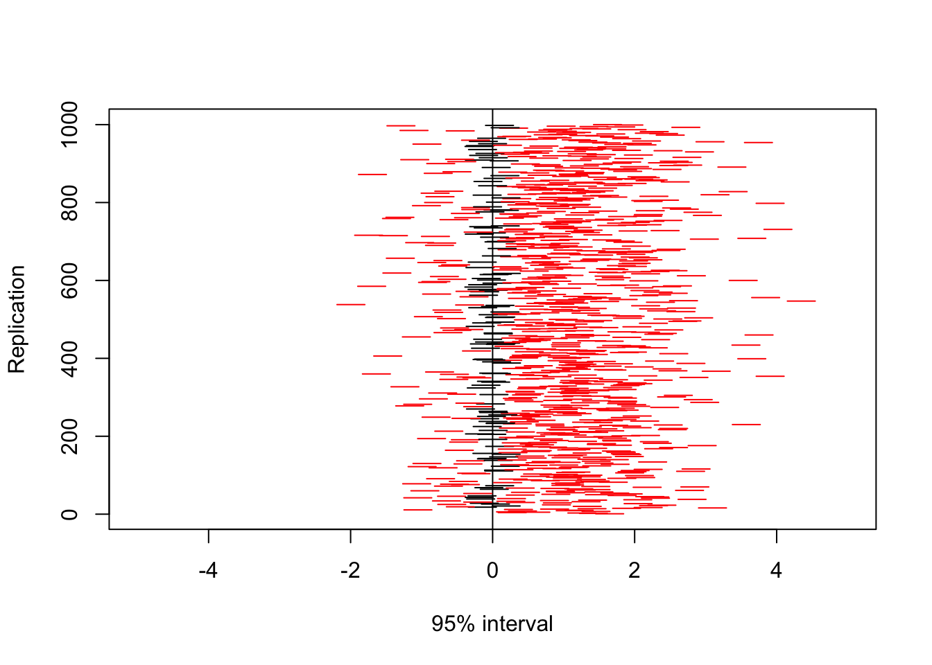
mean(L>0 | U<0)## [1] 0.885Better to double the effect size than to double the sample size. Standard errors of samples decrease with \(\sqrt{N}\)