Chapter 20 The Analysis Workflow

There are only two hard things in Computer Science: cache invalidation and naming things. –Phil Karlton

The first step in any project, no matter the size, is scoping the project in regards to what data sources are needed, what data needs to be captured, what kind of research quesxtion is being asked and what kind of analysis is expected (is it a formal report or simply the aggregate statistics or even just a “its going well keep it up”). One of the most overlooked components is the actual infrastructure of the project itself. This includes the file structure, the naming of the documents and even the structure of the report itself. While this often isn’t an issue for small teams working together, larger teams that work more collaboratively require rules of enghagement on these subjects to avoid stepping on each other and duplicating (or deleteing) anothers work. As such I feel that Institutional Researtchers should take a more industrial approach borrowed from software engineering and industrial data science teams. I will argue that by first ensuring that the right question is being asked and answer and through a common application of a project structure, a common reporting methodology and through the use of version control a better data product can be generated not only for the present problem but also provide a robust architecture for future knowledge sharing.

I will not lie, following this methodology is painful and slow. However this only lasts the first time. Whenenever you return to an analysis that was completed ad hoc and you find that you will have to completely re-create it, you will thank me for this moire rigourous approach. If you follow the process and always operate under the assumption that the same question will be asked again you will not regret it. Beyond this, the common structure creates an environbment where knowledge sharing becomes easy because everything follows a common approach. This helps not only the current team members but also makes onboarding of new personnell much easier.

20.1 Answering (and asking) the Right Question

The most important process is a workflow is to make sure that you are answering the correct question. Does this mean, “hey run a t-test on these two groups and tell me if there is a statistically significant difference.” No! In fact it is most important that a data scientist push back on the customer or the person who asked for such an analysis. The most important start and really the power of data science as a trade comes to pass when a question is asked. Data science is not the application of a principle at the request of another but an extention of the scientific process. This process must start with a well formed question and a hypothesis.

Pushing back and asking for the question behind the request is one of the hardest transitions for data scientists. Often you will be confronted with questions about the legitimacy of the data scientist pushing back. Just do what I ask could be the response. Here I argue it is first and foremost the ethical responsibility of the data scientist as a science to ask for the hypothesis that the individual is testing and what deeper question they seek to ask. This is science. It is testing hypothesis and askign broad questions. Secondly it results in a much more value added product at the end of the exploration and analysis. If the data scientist knows the question and the context of the question he or she can explore many types of tests and explore other confounders that may not have been included in the cookbook order request. As such is it paramount that a data scientist understand s the question.

20.1.1 The Right Question

Here it gets a little more challenging in that the data scientist must also ensure that the right question is being asked. The right question can be a little more subjective, but by understandign the context of the question the data scientist can help the customer understand what questions can be asked of the data available and what additional data would be needed. Additionally, the data scientist can help guide the discussion to understand if the framing of the question is statistically valid. This is especially important when the audience wishes to move beyond descriptive statistics and into making causal claims. One such example is having a customer ask if a certain class improved educations outcomes versus those who did not take the class. Important in this example is that academically at risk students are placed in this class by counselors in order to help adjustment to college. In this context the better question would be did this class improve education outcomes for students who were placed in the class versus those students who are similar to them (in which a technique like matched pairs or propensity score matching could be applied.) By ensuring that the right question is asked, the data scientist can help to ensure that the true research question is being answered in a robust and valid way.

20.2 A Common Project Structure

Each analysis should function like a consulting project with a highly regimeneted and organized and common structure. While in small IR organizations this approach can feel a bit heavy, it lends itself to some of the key points of both research and personel

• Reproducibility
• Easing Transitions

We live in a world where people move jobs. While academic turn over is not at the same rates as some other positions, the day will come when a new employee enters the office and another retires (or wins the lottery). When this happens if every project and analysiss that was ever completed in the office is completely different than the other then the new employee will spend the next year trying to figure out what was done in order to re-run old analysis. This is certainly non-optimal. As such is powerful to apply a common approach with the visision that eventually all projects will be handed off.

In addition having a common workflow facilitates code review wand sharing for the same reasons. If I name all my R functions as verbs and store then in the lib folder in each project then a colleuage can quickly see what I wrote. Additionbally, if I always specify the input and output parameters of the custom functon and add some unit tests to check for internal validity then the person coming to the code for the first time can debug issues or modify it quickly for a new analsysis.

Reproducibility refers to the ability to produce the same analysis with the same code and data. This is critical for any kind of environment where analysis is shared and desicisions are made. One of the worst possibilities is that you provide different answers with the same data and same methods to a decision maker. When this happens the entire organization loses credibility.

These conditions can all be ameliorated through the use of a common analysis structure. This is the rebar in the concrete.

20.2.1 Initiate with an project

I am a strong fan of the RStudio IDE. It provides a fantastic environment in which to do analysis both from the point of few of writing the function but also in structuring said analysis. MY recommendantion here is that each analysis starts with a new RStudio Project. The Rstudio project serves as an “anchor” for the analysis and provides a point for each new analyst to pick up the ball. Additionaly, the project structure always for the use of some relative references. These are incredibly handy when moving into the next recommendation for file organizaton and naming.

20.2.2 File Structure

Having a common file structure within the project provides a common understanding of where thigns should be. Similarly to putting your keys in a bowl by the door always having raw data in a data/ folder provides an easy way to find the common things. That being said for each project one should minimally find folders for:

• data
• munge
• src
• reports

Additionally one might find the need for the following:

• libs
• tests
• figures

In the main directory you should also have a README file that provides some orientation regarding the project and instructions. A neat way to initiate this is with usethis::use_readme_rmd

20.2.2.1 README

The README file is a necessary and often overlooked part of the project structure. It is in this file that you should orient the entire project. When did the project begin, what is the research question and the approach that you are going to use. It is a work in progress as the data science process is iterative but it should at least orient a new person to the project proper. When the project is completed you should review the README file and ensure that the high points of the analysis process have been touched. This is not a summary of the project; that is why you have a reports folder. It is instead a global orientation to the project, where things are located and helpful information. This is a critical introduction that makes handing a project off or re-laucnhing a simialr analysis much easier down the line.

20.2.2.2 Data

Unpacking these terms a little more, data is pretty self explantory. It is in this folder that you should put all of the data that is used in the analysis. The analysis springs from the data and so you should always find this folder in any analysis. This includes the flat csv files, excel files and any other raw data. In the case of pulling from a database my recommendation is to include in this folder the code used to call the data utilised in the analysis from the database. This will provide a robust and repeatable process for data storage and provenance. By provenance I eman here a versioning of the data. Compairosns can be completed between only and new data and can be checked in order to see what the changes were. This also aids in reproducibility because the data that drives the analysis is packaged with the analysis itself.

20.2.2.3 Munge

Munging is one of those domain specific words that I always use begrudgingly but it is in this folder that you should store scripts that deal specifically with the tidying, cleaning and reformatted of the raw data. These scripts should be thoroughly documented and commented in order to describve each transformation process. As a reminded the raw data is never to be modified so if there are any changes to the data that need to take place (cleaning up regular expression i.e. mispelled words or perhaps issues with encoding like dropping a leading zero in a character string that was read as a numeberic). Munging is often times 80% of the work of a data scientist and where most often errors are caught, correct and conversely made.

20.2.2.4 Src

Starting to get into the business of exploring that data and completing the analysis you should find these scripts in the src folder. This is a handy place to store the scripts and perhaps even the notebooks where the initial data exploration takes place. Additionalyl when it comes time this is the place to store the heavy analysis scripts. For instance I would store all of the jags models in this section. They would be documented. A nice touch here is to include a README document in this folder than explains generally what question each of the scripts is attempting to answer.

20.2.2.5 Reports

This is pretty explatory but it is in the reports section that all reports should be stored. This makes it easy to direct someone to the final reportings of the analysis without having them wade through your entire analysis (includign munging work) to find the conclusions. The rmardkown or bookdown frameworks provide a greate way to interleave code and text and present handsome reports and communication tools. Regardless of the method this should be where one can find the final report for the analysis.

20.2.2.6 Libs

Moving into the bonus or as needed folder is first lib/. The lib is a consolidated place to store any of the functions that have been created in the process of the analysis. The general rule is to create a function if you copy and paste your code more than twice. As such you will find yourself generating many functions if you follow that rule. If the function is something you use in many different analyses then perhapos it is time to wrap it into a package, but often times you just need a bespoke tool to deal with an issue at hand. As such you write a function and store it in this folder. It is important here to mention that each functon in this folder should have the complete roxygen headers. This includes the #' @param information which includes a function title, description, parameters used and the output of the function. This may seem like a bit of overdocumentation but it makes the functions easier to debug and move into a package if you use the function frequently enough to warrant doing so. Regardless, this folder provides a centralised location to store the custom function instead of leaving them burried in the munging scripts or the analysis scripts. This helps with debugging and is worth the extra effort when custom functions are needed.

20.2.2.7 Tests

20.2.2.7.1 Function Unit Testing

Testing is useful in two domains first the functions. IF you have written custom functions it is a good practice to include some unit tests to ensure that given a known input a known output comes out. For a silly example see my below new function which does an addition operation:

my_add <- function( x, y){
  out <- x + y
}

After I have carefully documented this function and stored it in my lib folder I want to write a test that ensure the function has the correct behaviour.

library(testthat)
test_that("Adding returns correct values", {
  expect_equal(my_add(1,2), 3)
  expect_equal(my_add(2,-1), 1)
  expect_equal(my_add(-1, -9), -10)
})

Using this testing I see that my function can provide outputs for positive and negative numbers when doing addition. But what about unknown values or strings?

test_that("Adding returns correct values", {
  expect_equal(my_add(1,NA), NA)
  expect_error(my_add(1, "A"))
})

This test throws an error stating that the function does not through the expected error. If I were to pass an NA to my function I would not get the expected response. This allows me the opportunity to go back and fix my function. Writing these kinds of unit tests for function may appear tedious but they often help you think through edge cases for your functions. While the above example is pretty trivial, often times one will find themselves writing complicated functioned that are critical to the sucess of the analysis. As such it is a good practice to think through these edge cases and ensure that proper unit testing is in place.

20.2.2.7.2 Data Unit Testing

Writing the tests for the custom function can be avoided. It is good software engineering practice to write out the unit testing operations. However, writing tests for the incoming data is often critical to a sucessful analysis. This is especially the case when the incoming data is coming from a data engineering pipeline and less often when it is coming in from static files like csvs.

Unit testing for data import is really ensuring that the data was imported correctly. Sometimes with the data import function, unless you explicitly specify the column types the program will make an estimate. It some cases these estimates will be incorrect and can leave you with issues. Additionally if you modify your code to add a new data set and suddenly find that soem downstream analysis and scripts are no longer executing you may spend your time looking for a bug in the analysis when the reality is that the data format changed. One way to avoid this major issues is to perform unit testing on the data input process. This can take the form of simply ensuring that the data is imported correctly and that it fits the expected limits. For example I want to ensure that my dataset does not have any NAs present. This can be especially true after I have munged that data as well.

assertthat::noNA(mtcars)

## [1] TRUE

Hooray! No NAs have been found. Additionally, I may want to check some additional features. The validate package is a wonderful tool for completing such analysis. In it you can supply some additional arguments.

library(validate)
validate::check_that(mtcars, mpg >0, disp >0, vs <= 1, wt >0)

## Object of class 'validation'
## Call:
##     validate::check_that(mtcars, mpg > 0, disp > 0, vs <= 1, wt > 
##     0)
## 
## Confrontations: 4
## With fails    : 0
## Warnings      : 0
## Errors        : 0

Additionally this package provides some nice graphics to visually display if an error occured. I have intentionally added a restrictive term to tthe validation set in order to show that this visually depicts that fourteen items valye the v3 test which is the vs < 0.5 test.

barplot(validate::check_that(mtcars, mpg >0, disp >0, vs < .5, wt >0))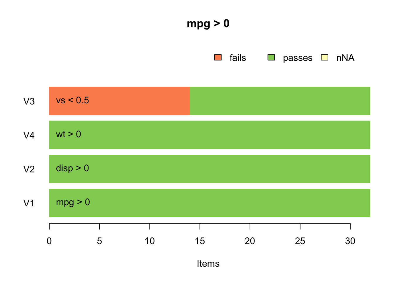

If I am interested in exploring this further I can look at the summary as well as the validater object itself

summary(validate::check_that(mtcars, mpg >0, disp >0, vs < .5, wt >0)) %>% 
  dplyr::filter(fails > 0)

##   name items passes fails nNA error warning expression
## 1   V3    32     18    14   0 FALSE   FALSE   vs < 0.5

This kind of input data unit testing is of the utmost importance and can provide a robust way to ensure that data is imported correctly.

20.2.2.7.3 Analysis Unit Testing

In the course of any analysis assumptions are typically made about the distribvution. For instance a normal distribution may be assumed so that a student’s t-test can be performed. This hypothesis may be tested with a Shapiro-Wilk test for normallity initially. However, in the course of time new data may become available. This data level testing must be completed again because it could be possible that the data are no longer normal and a different statistical test needs to be performed. This is a simple example but one that happens quite frequently. These kinds of testing must be built into the analysis and through warnings if something has changed. Or more provocatively a robust analysis is one in which these fail safes are built in and a more appropriate method is selected automatically. Let’s step though an example.

My data enters and I perform some testing to test for normallity to ensure that I can perform a t-test. With a p-value > 0.05 I can make the assumption that the data are normal and I can go ahead with my testing.

df_1 <- rnorm(100, 50, 1)
df_2 <- rnorm(100, 59, 1)

(shapiro.test(df_1))

## 
##  Shapiro-Wilk normality test
## 
## data:  df_1
## W = 0.97887, p-value = 0.1085

(shapiro.test(df_2))

## 
##  Shapiro-Wilk normality test
## 
## data:  df_2
## W = 0.99295, p-value = 0.8849

t.test(df_1, df_2)

## 
##  Welch Two Sample t-test
## 
## data:  df_1 and df_2
## t = -72.577, df = 197.8, p-value < 2.2e-16
## alternative hypothesis: true difference in means is not equal to 0
## 95 percent confidence interval:
##  -9.360403 -8.865185
## sample estimates:
## mean of x mean of y 
##  49.98522  59.09801

Now completing my t-test I can confidently say that these two samples are in fact different with a p-value of less than 0.05.

But what it new data are provided from a third machine. I have built a robust analysis process so I just add the data and change one line of code to do my testing.

df_3 <- rgamma(100, 54, 1.5)
t.test(df_1, df_3)

## 
##  Welch Two Sample t-test
## 
## data:  df_1 and df_3
## t = 29.379, df = 106.83, p-value < 2.2e-16
## alternative hypothesis: true difference in means is not equal to 0
## 95 percent confidence interval:
##  12.65964 14.49172
## sample estimates:
## mean of x mean of y 
##  49.98522  36.40954

But wait, are my data truly normal? Should I just assume that they are without having any kind of check in place? No.

shapiro.test(df_3)

## 
##  Shapiro-Wilk normality test
## 
## data:  df_3
## W = 0.98759, p-value = 0.4783

dplyr::select

## function (.data, ...) 
## {
##     UseMethod("select")
## }
## <environment: namespace:dplyr>

Running the Shapiro Wilk test you find that the new data are not normal, they follow a gamma distribution. As such a t-test is no longer the most appropriate test and a wilcon test should be used (if we are following a frequentist analysis). Luckily the answer is the same in this case, but it others you might not be so lucky.

While statisticians make strong assumoptions when they choose a model. This is part of the process. As such we should build tests in place that ensure that in the presence of new data these assumptions are tested and confirmed. A simple example a unit test in this case would be a nice function

check_normality <- function(df){
  p.value <- broom::tidy(shapiro.test(df))$p.value
  if(p.value <= 0.05){ warning("Imported data is not normal, check QQ Plot")} else{
    message("Data passed")
  }
}

We can then apply this function to our new data:

check_normality(df_3)

## Data passed

And it provides our error message. This kind of foresight to design testing into the modeling process is hugely important and often underrated. You put a lot of thought into your model selection strategy. It is good to fortify your assumptions with these modeling unit checks to ensure that they are robust in the face of new data.

20.2.2.8 Figures

20.2.3 Function Writing

20.2.3.1 Custom APIs

20.3 Version Control

I think I need to start with a relevent cartoon.

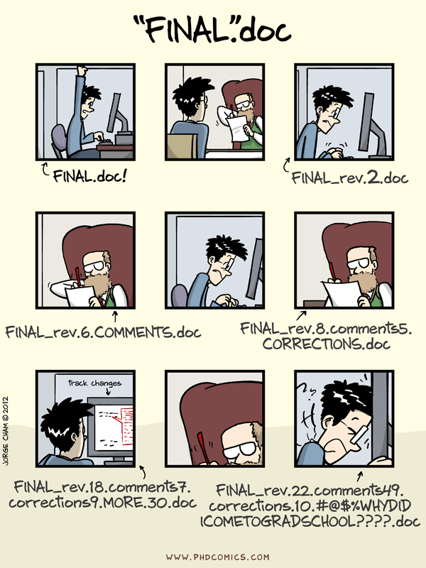
Who hasn’t been in a situatation where what you think is the “final” draft of something because the first in a new string of “final” edits? This might work for a few times (like writing your thesis at University), but when you are in an institition where you are generating a lot more frequent documents and analysis this kind of workflow just won’t work. You can’t have thirty different documents all with the same content floating on a shared drive. When you are in a business environment doing this is dangerous as the wrong report might get out. People may read something that wasn’t ready. Now confusion is sown and credibility damaged. This is obviously not the best approach. Enter version control.

Verion control is a way to organize and well, version , your analysis and scripts. It works best on plain text files like those writting in any command line programmiong language. In fact the “git” version control system originated as a way to version code for the development of the Linux operating system. Git is one of several version control systems, but it is very popular. In this system you can make changes, commit them (log a version of them) and then pull them into a “branch” or draft. The main branch (think of this as the production ready/ ready to be output) can remain unchanged until the different drafts are accepted and combined through a pull request and associated merge. Git nicely stores all the commit points so you have a running log of who changed what and when. If a change proves to be bad (or catostrophic) then you can unmerge that code and have the code restore.

Versioning helps with a few different fronts

1. Versioning This is relatively straight forward; versioning systems help you to understand what version are active, what are under development and understand what changed between the different version. It provides a clear evolution to the current master branch as well as the other branches exist. The provenance of the code that generated an analysis is essential. By having this rebust versioning there is a clear vision of what is the final version.

2. Collaboration By moving to version control it makes collaboration much easier. Now multiple people can be working simultaneously on different branchs of the analysis or documentation. After each is done then they can be merged together into a master branch. There is no confusion about who is working on what. Differences between the different collaboror’s documents can easily be shared. If you are using a service like github to host the repository of code you can even begin to use “issues” to track requests for changes or new additions to the code. Here you can also assign others issues to resolve or new parts of the analysis to write.

PICTURE

3. Sharing Github especially provides a great way to share data and analysis. It is a hosting site that allows for others to cloan a repository and do their own analysis. To stand of the shoulders of giants by taking existing code that has already been shared and enhancing it, learning from it and hopefully adding to it. This cannot be underscored enough. Sharing is vital to science and research, assuming that it can be shared within the restrictions of FERPA and IRB guidelines. Even if the data is protected if the analysis could be interesting to the community it can be shared.

Entire books have been written on this subject and I daresay I did not do the topic justice. If you are interested in more please see Jenny Bryan’s Happy Git with R.