Chapter 12 Dealing with Survey Data
Surveyes are a powerful tool that can are often found in Institituional Research. These surveys can come in the form of the typicaly Higher Education Research Initiative (HERI) among other more custom surveyes that administered at the university locally. Surveys can provide both quantitative information, especially regarding metrics that are not already built into the school’s data tracking systems. These include noncognitive constructs, opinion polls.
Surveyes offer a critical insight into the the minds of the users and often complement the more readily available information. These survey scores where allowed can then be integreated with any kind of analaysis alogirthms and may unearth some interesting trends.
12.1 Survey Analysis
Survey analysis is an entire subdiscipline of statistics with many books written on the topic. While a survey of the field of survey analysis is not the purpose of this book, it is worth noting that there are many good resources available out there. My personal favourite is Thomas Lumley’s Complex Survey Analysis with R. While we won’t be coming the deoth of survey analysis it is important as a researcher to be aware of at least some concepts.
12.1.1 Simple Random Sample
Simple random samples are random, but often not simple. However the idea of random sampling is attractive because randomization helps to reduce some variation. It also should generate an unbiased estimator.
12.1.2 Stratified Random Sample
12.1.3 Post Stratification
Post stratification is a useful tool that can be performed after the survey has been conducted. When coming the survey respondants to your global population statistics you might find that certain groups are over represented. As such you will need to downweight the responses for those who are over represented in the survey and upweight those who did not have response rates representaive of their population statistics. This is called post stratification or Mr P.
An excellent resource for doing this type of work is the survey package from Thomas Lumley. An example could be as follows. A survey was collected from students from a University. However, upon review more females than males responded. Additionaly, one ethnic group responded at a much lower rate. When reporting the survey scores it is important to post stratify for these differences otherwise the survey means that you present will not be representive of the population. Let’s take the survey data from the MASS package as our example. We will look at gender or biological gender first.
library(survey)
df <- (MASS::survey) %>% na.omit()
prop.table(table(df$Sex))
##
## Female Male
## 0.5 0.5This data indcates that we have an equal split of males and females in the survey responses. However, what if the true population statistics were 55% females and 45% female. We can correct for this using the survey package.
First we need to create the survey design object. This is a special R object that has more metadata. It also helps us perform transformations. First we must create the unweighted survey design object.
survey_design_unweighted <- svydesign(ids = ~1, data =df)## Warning in svydesign.default(ids = ~1, data = df): No weights or
## probabilities supplied, assuming equal probabilityThe survey package passes a warning that it will assume equal probabilities since we did not provide it with any additional information. This is ok and expecyed for now. Now we need to create our marginal distributions. Because we know the populations of students at the school is closer to a 55%/45% breakdown between females and males we can pass this to our survey design object, If we were surveying a different population we could use census statistics or other publically available information to set up our marginal distribution.
Now let’s apply our survey correction.
(gender_dist <- data.frame(Sex = c("Female", "Male"), Freq = round(nrow(df) * c(.55, .45),0)))## Sex Freq
## 1 Female 92
## 2 Male 76Now we can post-stratify on this metric.
survey_design_weighted <- postStratify(survey_design_unweighted, ~Sex, gender_dist)Now we can see the impact of this post-stratification.
svymean(~Height, survey_design_unweighted)## mean SE
## Height 172.48 0.7684svymean(~Height, survey_design_weighted)## mean SE
## Height 171.82 0.5384You can see from this simple post stratification that both the mean and the standard error were reduced. The effect of correcting is both a lower error rate as well as a more representative mean Height in this instance. But what if we have more than one marginal distribution which we want to post stratify by? Now we move into survey raking. For the sake of our example lets assume that we also need to correct for left-handed ness.
prop.table(table(df$W.Hnd))##
## Left Right
## 0.07142857 0.92857143A study has shown that the true population of left handed people is closer to 10% so we under sampled left handed people. Let’s correct for this and for gender.
Similar to before we need to set up our marginal distribution.
(handed <- data.frame(W.Hnd = c("Left", "Right"), nrow(df) * c(.1, .9)))## W.Hnd nrow.df....c.0.1..0.9.
## 1 Left 16.8
## 2 Right 151.2Now we will use a survey rake function to apply our two different marginal distributions to our unweighted survey object.
survey_design_rake <- rake(survey_design_unweighted, sample.margins = list(~Sex, ~W.Hnd), population.margins = list(gender_dist,handed))Now we can look at our new survey object. We can inspect the extent of the weighting to see if they are reasonable. In this case they appear to be reasonable for our sample with some samples being down-weighted to 0.87 and the maximum upweighting to 1.56. Typically these values are between 0.3 and 3. These can be controlled with the trimWeights function.
summary(weights(survey_design_rake))## Min. 1st Qu. Median Mean 3rd Qu. Max.
## 0.8706 0.8706 1.0654 1.0000 1.0654 1.5671Now let’s see how our new survey design object works.
svymean(~Height, survey_design_rake)## mean SE
## Height 171.91 0.5454This example illustrates the power of post stratification. This kind of analysis must be done on surveys where there were no stratification plans in place. This is also a good strategy when dealing with response surveys. This helps to control for over-representation of certain groups in the response rate. However, no amount of post-strateification can correct for missing populations. If a group did not have a significant number of respondants there is no way to post stratify on that variable. Analysis can still be done, but it must be understood that the survey does not have complete coverage and can’t speak to that missing group.
12.1.4 Finite Population Corrections
When you are dealing with a finite population (or at least finite in terms of statistics) there is a correction that can be done to reduce the variability. This is because samples of roughly 10% of the total population or greater represent a large sampling fraction and can take advanatage of the fact that a larger sample of the population has been sampled and thus the variability or measurement error begins to decrease.
library(srvyr)
library(survey)
library(dplyr)
data(api)

strat_design_srvyr <- apistrat %>%
  as_survey_design(1, strata = stype, fpc = fpc, weight = pw,
                variables = c(stype, starts_with("api")))

strat_design_srvyr <- strat_design_srvyr %>%
  mutate(api_diff = api00 - api99) %>%
  rename(api_students = api.stu)

strat_design_srvyr %>%
  summarize(api_diff = survey_mean(api_diff, vartype = "se"))
## # A tibble: 1 x 2
## api_diff api_diff_se
## <dbl> <dbl>
## 1 32.9 2.05strat_design_srvyr %>%
summarise(api_diff_uw = unweighted(mean(api_diff)))## # A tibble: 1 x 1
## api_diff_uw
## <dbl>
## 1 28.012.1.5 Finite Population Correction
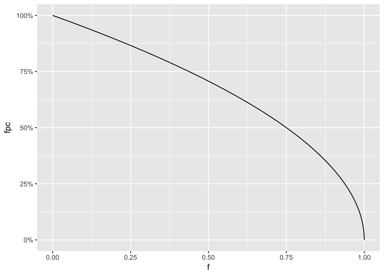
When sampling without replacement there is a term that must ve added to the analysis called the finite population correction. This term allows for reducing the predicted standard errors and thus the variance by considering the population that is known. Thus the more samples you have from the population the less variance there is. Often with large surveys like the census and national opinion polls this fpc adjustment can be negligated as it tends to zero with large samples. However, in instances where there is a small population and a large survey response rate it can help to reduce the estimated standard errors.
\[Sampling Fraction =\frac{n}{N}\] \[fpc = (1- \frac{n}{N})\] Effect of fpc on standard error is \(1 - \frac{f}{2}\) and then
12.1.6 But is it representative
12.1.7 Non-Response Bias
12.1.8 Confirmation Bias
12.2 Constructs
- IRT
- FA
- PCA