ggdist and Epidemic Curves

This post explores using tools to summarise curves rather than fixed time summary methods. This includes using odin and ggdist to explore the risk of underestimating epidemic curves.

pandemic
scenarios
curve statistics
Author
Affiliation
Published

August 9, 2020

library(ggplot2)
library(dplyr)

Attaching package: 'dplyr'
The following objects are masked from 'package:stats':

    filter, lag
The following objects are masked from 'package:base':

    intersect, setdiff, setequal, union
library(tidyr)
library(ggdist)
library(odin)
theme_set(theme_minimal())

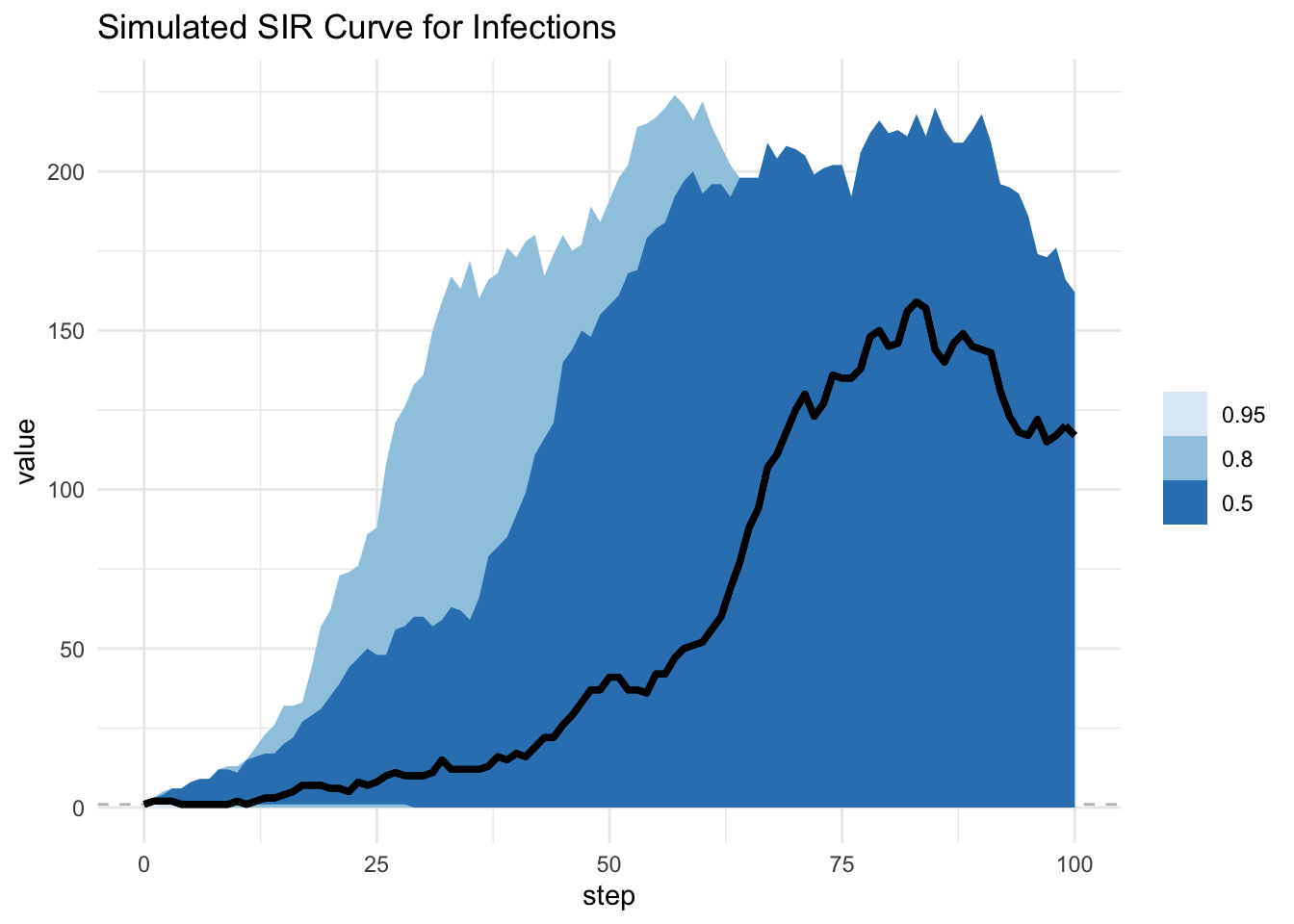
This little post is based on a recent paper by Juul et al. (2020). For infectious disease modelling we are often running many scenarios through the models. Why? Because there are many parameters to estimate, but very few things that we actually observe (cases by day or incidence) so in some sense our models all suffer from identifiability issues. Additionally, many of the parameters that we do measure have some uncertainty around them. For this reason it is very common to run models with different parameters estimates or distributions in order to understand a range of possible values. A simple way to summarise these models is through point-wise quantiles through time. The genius of Juul’s paper is that this can underestimate many outcomes because it might pick up the beginning of one epidemic curve and miss the peak.

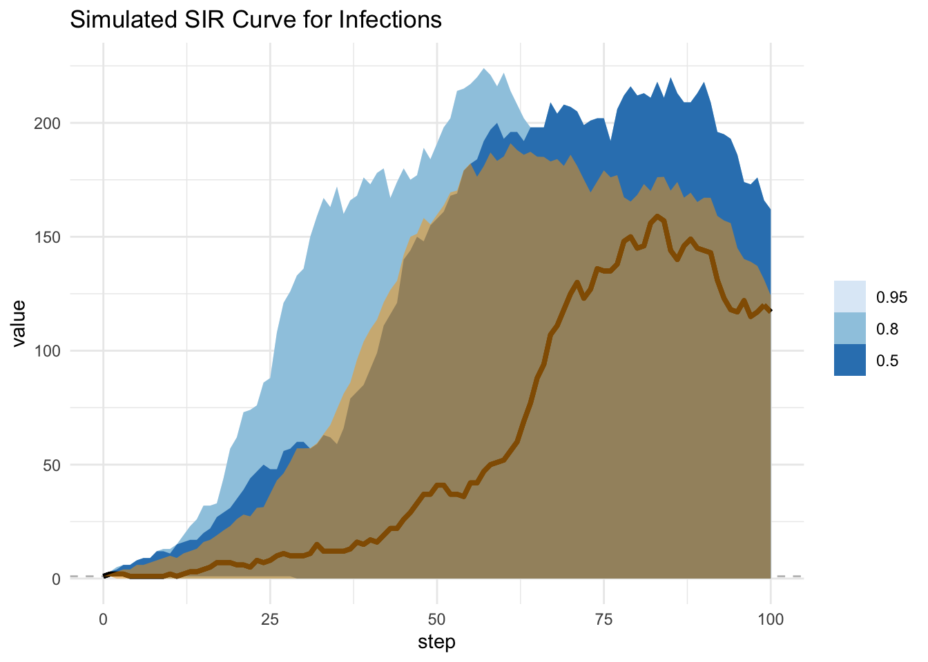
Enter curve estimates. These measures actually look at the curves proper through the trajectory rather than at discrete time points. Here we can rank the entire curve and capture the contribution of the curve rather than the point-wise estimate.

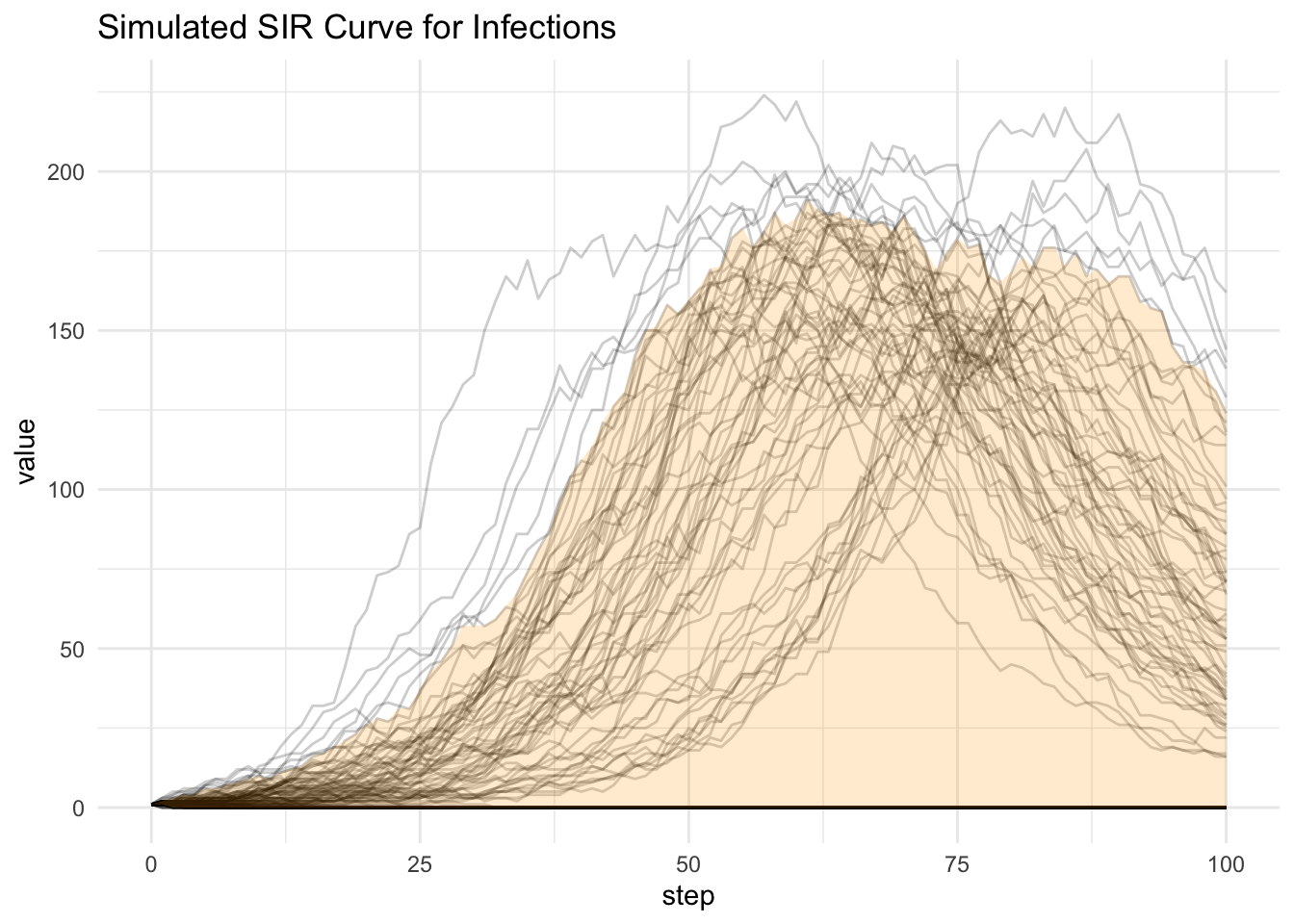
To see this let’s run a simple example from the odin package (FitzJohn 2019). Additionally, the amazing ggdist (Kay 2020) provides an easy way to summarise curves.

sir_model <- system.file("examples/discrete_stochastic_sir_arrays.R", package = "odin")

writeLines(readLines(sir_model))
## Core equations for transitions between compartments:
update(S[]) <- S[i] - n_SI[i]
update(I[]) <- I[i] + n_SI[i] - n_IR[i]
update(R[]) <- R[i] + n_IR[i]

## Individual probabilities of transition:
p_SI[] <- 1 - exp(-beta * I[i] / N[i])
p_IR <- 1 - exp(-gamma)

## Draws from binomial distributions for numbers changing between
## compartments:
n_SI[] <- rbinom(S[i], p_SI[i])
n_IR[] <- rbinom(I[i], p_IR)

## Total population size
N[] <- S[i] + I[i] + R[i]

## Initial states:
initial(S[]) <- S_ini
initial(I[]) <- I_ini
initial(R[]) <- 0

## User defined parameters - default in parentheses:
S_ini <- user(1000)
I_ini <- user(1)
beta <- user(0.2)
gamma <- user(0.1)

## Number of replicates
nsim <- user(100)
dim(N) <- nsim
dim(S) <- nsim
dim(I) <- nsim
dim(R) <- nsim
dim(p_SI) <- nsim
dim(n_SI) <- nsim
dim(n_IR) <- nsim
x <- odin(sir_model)
Loading required namespace: pkgbuild
Generating model in c
Re-compiling discrete.stochastic.sir.arrays30f32291
* installing *source* package ‘discrete.stochastic.sir.arrays30f32291’ ...
** using staged installation
** libs
/usr/local/opt/llvm/bin/clang  -I"/usr/local/Cellar/r/4.1.2/lib/R/include" -DNDEBUG   -I/usr/local/opt/gettext/include -I/usr/local/opt/readline/include -I/usr/local/opt/xz/include -I/usr/local/include   -fPIC  -g -O3 -Wall -pedantic -std=gnu99 -mtune=native -pipe -c odin.c -o odin.o
/usr/local/opt/llvm/bin/clang  -I"/usr/local/Cellar/r/4.1.2/lib/R/include" -DNDEBUG   -I/usr/local/opt/gettext/include -I/usr/local/opt/readline/include -I/usr/local/opt/xz/include -I/usr/local/include   -fPIC  -g -O3 -Wall -pedantic -std=gnu99 -mtune=native -pipe -c registration.c -o registration.o
/usr/local/opt/llvm/bin/clang -dynamiclib -Wl,-headerpad_max_install_names -undefined dynamic_lookup -single_module -multiply_defined suppress -L/usr/local/Cellar/r/4.1.2/lib/R/lib -L/usr/local/opt/gettext/lib -L/usr/local/opt/readline/lib -L/usr/local/opt/xz/lib -L/usr/local/lib -o discrete.stochastic.sir.arrays30f32291.so odin.o registration.o -L/usr/local/Cellar/r/4.1.2/lib/R/lib -lR -lintl -Wl,-framework -Wl,CoreFoundation
installing to /private/var/folders/0x/6bnjy4n15kz8nbfbbwbyk3pr0000gn/T/RtmpWCtpbh/devtools_install_10f003a777ae8/00LOCK-file10f007037fdf1/00new/discrete.stochastic.sir.arrays30f32291/libs
** checking absolute paths in shared objects and dynamic libraries
* DONE (discrete.stochastic.sir.arrays30f32291)
ℹ Loading discrete.stochastic.sir.arrays30f32291
fit <- x()
Warning: 'x(...)' is deprecated; please use 'x$new(...)' instead
sampz <- as.data.frame(fit$run(step = 100))

Now that we have values, a simple analysis would look like the following:

val_long <- sampz %>% 
  select(step, contains("I")) %>% 
  tidyr::gather(key, value, -step) %>% 
  mutate(.draw = readr::parse_number(stringr::str_extract(key,"\\d+")))

sumz_point <- val_long %>% 
  group_by(step) %>% 
  summarise(q05 = quantile(value, probs = .05),
            q95 = quantile(value, probs = .95))

val_long %>% 
  ggplot(aes(step, y = value, group = .draw))+
  geom_line(alpha = .2)+
  geom_ribbon(data = sumz_point, 
              aes(x = step, ymin = q05, ymax = q95), 
              inherit.aes = FALSE, fill = "orange", alpha =.2)+
  labs(
    title = "Simulated SIR Curve for Infections"
  )

If we take the curve distribution approach we can see the following

p <- val_long %>% 
  group_by(step) %>%
  curve_interval(value, .width = c(.5, .8, .95)) %>%
  ggplot(aes(x = step, y = value)) +
  geom_hline(yintercept = 1, color = "gray75", linetype = "dashed") +
  geom_lineribbon(aes(ymin = .lower, ymax = .upper)) +
  scale_fill_brewer() +
  labs(
    title = "Simulated SIR Curve for Infections"
  )

p

Now when we lay these ontop of one another, we see the issue with using the time interval method:

p+
  geom_ribbon(data = sumz_point, 
              aes(x = step, ymin = q05, ymax = q95), 
              inherit.aes = FALSE, fill = "orange", alpha =.5)

We see that using the fixed time method we underestimate the peak much of the time! This is very dangerous and important when setting policy and establishing needs.

References

FitzJohn, Rich. 2019. Odin: ODE Generation and Integration. https://CRAN.R-project.org/package=odin.
Juul, Jonas L., Kaare Græsbøll, Lasse Engbo Christiansen, and Sune Lehmann. 2020. “Fixed-Time Descriptive Statistics Underestimate Extremes of Epidemic Curve Ensembles.” arXiv:2007.05035 [Physics, q-Bio, Stat], July. http://arxiv.org/abs/2007.05035.
Kay, Matthew. 2020. ggdist: Visualizations of Distributions and Uncertainty. https://doi.org/10.5281/zenodo.3879620.

Reuse

Citation

BibTeX citation:
@online{dewitt2020,
  author = {Michael DeWitt},
  title = {Ggdist and {Epidemic} {Curves}},
  date = {2020-08-09},
  url = {https://michaeldewittjr.com/programming/2020-08-09-ggdist-and-epidemic-curves},
  langid = {en}
}
For attribution, please cite this work as:
Michael DeWitt. 2020. “Ggdist and Epidemic Curves.” August 9, 2020. https://michaeldewittjr.com/programming/2020-08-09-ggdist-and-epidemic-curves.