Speeding Things Up with Rcpp

Likelihood

\[f(x_i,...,x_n|\theta)=\frac{1}{\pi^n(1+\Pi_{i=1}^n(x_i-\theta)^2)} \ for \ -\infty<x<\infty\]

Prior Distribution

\[p(\theta)=\frac{1}{\sqrt{2\pi}}exp(-\theta^2/2)\]

M-H Sampler

Now to build the Metropolis Hastings sampler we build the corresponding R functions.

prior <- function(theta){
  1/sqrt(2*pi)*exp(-theta^2/2)
}

And an associated check to make sure it is providing logical values:

(test_prior <- prior(theta = .1))

[1] 0.3969525

Then we build the likelihood function. In order to prevent integer underflow I have converted the function to log-likelihood. I then exponentiate the final value. The log-likelihood is then describved as

\[l(x_i,...x_n|\theta) = log(1) - (n\log(pi)+\Sigma_{i=1}^nlog(1+(x_i-\theta)^2))\]

The value from the log-likelihood can then be exponentiated in order to arrive at the likelihood.

likelihood <- function(x, theta){
  if(!is.vector(x)){
    stop("Please supply a vector to this function")
  }
  # Log-likelihood
  a <- log(1)-(length(x)*log(pi) + sum(log(1+(x-theta)^2)))
  
  # Convert to likelihood
  exp(a)

}

And finally we build the sampler.

theta_sampler <- function(x, niter, theta_start_val, theta_proposal_sd){
  
  theta <- rep(0, niter)
  theta[1] <- theta_start_val
  
  for(i in 2:niter){
    current_theta <- theta[i-1]
    
    # Random Step
    new_theta <- current_theta + rnorm(1,0, theta_proposal_sd)
    
    # MH Ratio
    r <- prior(theta = new_theta) * likelihood(theta = new_theta, x = x)/
      (prior(theta = current_theta)* likelihood(theta = current_theta, x = x))
    
    # Decide to keep proposed theta or take a step
    if(runif(1)<r){
      theta[i] <- new_theta
    } else{
      theta[i] <- current_theta
    }
  }
  return(theta)
}

We can then sample from the posterior distribution given the initial values and our data.

set.seed(336)
out <- theta_sampler(x = x, niter = 5000, theta_start_val = 0, theta_proposal_sd = .5)

We can then graph our associated draws.

hist(out[1000:5000], 
     main = "Histogram of Posterior Draws of theta", 
     xlab = expression(Posterior~Value~of~theta),
     breaks = 30)
abline(v = mean(out[1000:5000]), col = "red", lwd = 2)

The posterior mean of \(\theta\) is:

mean(out)

[1] 0.1280924

C++ Code

This code is nearly identical to the R code, just utilising C++. Astute readers will see that I really could drop some of the constants in the prior and the likelihood function because they will fall out when calculating the MH ratio, r. Additionally, it is worth noting that I have converted the equations to a log scale to avoid computations on very small numbers.

writeLines(readLines("mh_sampler.cpp"))

#include <Rcpp.h>
using namespace Rcpp;

// [[Rcpp::export]]
double Priorcpp(double theta) {
  return 1/sqrt(2*M_PI)*exp(-pow(theta,2)/2);
}

// [[Rcpp::export]]
double Likelihoodcpp(NumericVector x, double theta) {
  double likelihood;
  double loglike;
  int n = x.size();
  
  loglike = log(1) - (n*log(M_PI)+sum(log(1+pow((x-theta),2))));
  likelihood = exp(loglike);
  return likelihood;
}

// [[Rcpp::export]]

NumericVector make_posterior(NumericVector x, int niter, 
                             double theta_start_val, double theta_proposal_sd){
  NumericVector theta(niter);
  double current_theta;
  double new_theta;
  double r;
  double rand_val;
  double thresh;
  
  theta[0] = theta_start_val;
  
  for(int i = 1; i < niter; i++){
    
    current_theta = theta[i-1];
    
    rand_val = rnorm(1,0, theta_proposal_sd)[0];
    
    new_theta = current_theta + rand_val;
    
    
    r = Priorcpp(new_theta) * Likelihoodcpp(x, new_theta)/
      (Priorcpp(current_theta)* Likelihoodcpp(x, current_theta));
    
    
    thresh = runif(1)[0];
    
    theta[i] = new_theta;
    
    
    if(thresh<r){
      theta[i] = new_theta;
    } else{
      theta[i] = current_theta;
    }
    
    
  }
  return theta;
}

Compilation and Testing

Now we need to compile the functions.

library(Rcpp)
Rcpp::sourceCpp("mh_sampler.cpp")

First we meed to test that the prior and likelihood functions return equivalent values between base R and C++.

all.equal(
prior(theta = .1),
Priorcpp(theta = .1)
)

[1] TRUE

So Priors are returning the same values.

all.equal(
likelihood(x = x, .1),
Likelihoodcpp(x = x, theta = .1)
)

[1] TRUE

The likelihoods are returning the samples values. Now we have confidence that our C++ function is returning the same values.

Inference using C++

Now we can go ahead and draw from the posterior distribution using our sampler.

set.seed(336)
out2 <- make_posterior(x = x, niter = 5000, theta_start_val = 0, 
                       theta_proposal_sd = .5)

hist(out2[1000:5000],
     main = "Histogram of Posterior Draws of theta", 
     xlab = expression(Posterior~Value~of~theta),
     breaks = 30)
abline(v = mean(out2[1000:5000]), col = "red", lwd =2)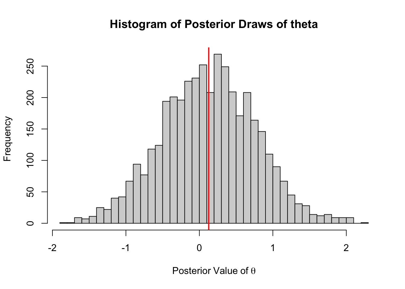

The mean value, 0.127 is very similar to the base R version (some differences could be some differences in the random number generators used). However, we we compare the benchmark times we see that the C++ version of the sampler is roughly 20x faster.