Insufficient Statistics - Hierarchical Time Series with hts

Mission

The mission is to reproduce the figures in the following article:

https://cran.r-project.org/web/packages/hts/vignettes/hts.pdf

Load Required Libraries

library(hts)

Loading required package: forecast

Registered S3 method overwritten by 'quantmod':
  method            from
  as.zoo.data.frame zoo

Note on Formatting Data

This is important to understand in regard to how to format the data.

# bts is a time series matrix containing the bottom-level series
# The first three series belong to one group, and the last two
# series belong to a different group
# nodes is a list containing the number of child nodes at each level.
bts <- ts(5 + matrix(sort(rnorm(500)), ncol=5, nrow=100))

y <- hts(bts, nodes=list(2, c(3, 2)))

Since argument characters are not specified, the default labelling system is used.

The Data

infantgts

Grouped Time Series 
4 Levels 
Number of groups at each level: 1 2 8 16 
Total number of series: 27 
Number of observations per series: 71 
Top level series: 
Time Series:
Start = 1933 
End = 2003 
Frequency = 1 
 [1] 4426 4795 4501 4813 4572 4627 4726 4897 5367 5435 5458 4819 4741 5143 5231
[16] 4978 4621 4672 4910 4823 4743 4546 4571 4630 4751 4586 4915 4667 4700 4861
[31] 4652 4403 4124 4065 4205 4293 4507 4620 4809 4465 4088 3974 3341 3161 2834
[46] 2732 2557 2438 2365 2485 2349 2184 2473 2162 2131 2143 2018 2149 1851 1848
[61] 1598 1524 1466 1467 1352 1261 1413 1292 1313 1271 1207

Use a bottom’s up forcasting method. There are several options from which to choose:

comb optimal combination
bu bottom’s up
mo middle out forecast
tdgsa Top-down forecasts based on the average historical proportions (Gross-Sohl method A)
tdgsf same as above but with averages
tdfp top down forecast using proportions

# Forecast 10-step-ahead using the bottom-up method
infantforecast <- forecast(infantgts, h=10, method="bu")

Warning in FUN(X[[i]], ...): partial argument match of 'freq' to 'frequency'

Warning in FUN(X[[i]], ...): partial argument match of 'freq' to 'frequency'

Warning in FUN(X[[i]], ...): partial argument match of 'freq' to 'frequency'

Warning in FUN(X[[i]], ...): partial argument match of 'freq' to 'frequency'

Warning in FUN(X[[i]], ...): partial argument match of 'freq' to 'frequency'

Warning in FUN(X[[i]], ...): partial argument match of 'freq' to 'frequency'

Warning in FUN(X[[i]], ...): partial argument match of 'freq' to 'frequency'

Warning in FUN(X[[i]], ...): partial argument match of 'freq' to 'frequency'

Warning in FUN(X[[i]], ...): partial argument match of 'freq' to 'frequency'

Warning in FUN(X[[i]], ...): partial argument match of 'freq' to 'frequency'

Warning in FUN(X[[i]], ...): partial argument match of 'freq' to 'frequency'

Warning in FUN(X[[i]], ...): partial argument match of 'freq' to 'frequency'

Warning in FUN(X[[i]], ...): partial argument match of 'freq' to 'frequency'

Warning in FUN(X[[i]], ...): partial argument match of 'freq' to 'frequency'

Warning in FUN(X[[i]], ...): partial argument match of 'freq' to 'frequency'

Warning in FUN(X[[i]], ...): partial argument match of 'freq' to 'frequency'

Now we can plot them:

# plot the forecasts including the last ten historical years
plot(infantforecast, include=2)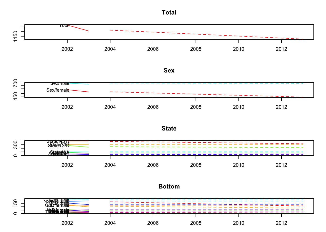

allts_infant <- aggts(infantgts)
allf <- matrix(nrow=10, ncol=ncol(allts_infant))
# Users can select their preferred time-series forecasting method
# for each time series
for(i in 1:ncol(allts_infant)){
  allf[,i] <- forecast(auto.arima(allts_infant[,i]), h=10, PI=FALSE)$mean
}

Warning in forecast.forecast_ARIMA(auto.arima(allts_infant[, i]), h = 10, : The
non-existent PI arguments will be ignored.

Warning in forecast.forecast_ARIMA(auto.arima(allts_infant[, i]), h = 10, : The
non-existent PI arguments will be ignored.

Warning in forecast.forecast_ARIMA(auto.arima(allts_infant[, i]), h = 10, : The
non-existent PI arguments will be ignored.

Warning in forecast.forecast_ARIMA(auto.arima(allts_infant[, i]), h = 10, : The
non-existent PI arguments will be ignored.

Warning in forecast.forecast_ARIMA(auto.arima(allts_infant[, i]), h = 10, : The
non-existent PI arguments will be ignored.

Warning in forecast.forecast_ARIMA(auto.arima(allts_infant[, i]), h = 10, : The
non-existent PI arguments will be ignored.

Warning in forecast.forecast_ARIMA(auto.arima(allts_infant[, i]), h = 10, : The
non-existent PI arguments will be ignored.

Warning in forecast.forecast_ARIMA(auto.arima(allts_infant[, i]), h = 10, : The
non-existent PI arguments will be ignored.

Warning in forecast.forecast_ARIMA(auto.arima(allts_infant[, i]), h = 10, : The
non-existent PI arguments will be ignored.

Warning in forecast.forecast_ARIMA(auto.arima(allts_infant[, i]), h = 10, : The
non-existent PI arguments will be ignored.

Warning in forecast.forecast_ARIMA(auto.arima(allts_infant[, i]), h = 10, : The
non-existent PI arguments will be ignored.

Warning in forecast.forecast_ARIMA(auto.arima(allts_infant[, i]), h = 10, : The
non-existent PI arguments will be ignored.

Warning in forecast.forecast_ARIMA(auto.arima(allts_infant[, i]), h = 10, : The
non-existent PI arguments will be ignored.

Warning in forecast.forecast_ARIMA(auto.arima(allts_infant[, i]), h = 10, : The
non-existent PI arguments will be ignored.

Warning in forecast.forecast_ARIMA(auto.arima(allts_infant[, i]), h = 10, : The
non-existent PI arguments will be ignored.

Warning in forecast.forecast_ARIMA(auto.arima(allts_infant[, i]), h = 10, : The
non-existent PI arguments will be ignored.

Warning in forecast.forecast_ARIMA(auto.arima(allts_infant[, i]), h = 10, : The
non-existent PI arguments will be ignored.

Warning in forecast.forecast_ARIMA(auto.arima(allts_infant[, i]), h = 10, : The
non-existent PI arguments will be ignored.

Warning in forecast.forecast_ARIMA(auto.arima(allts_infant[, i]), h = 10, : The
non-existent PI arguments will be ignored.

Warning in forecast.forecast_ARIMA(auto.arima(allts_infant[, i]), h = 10, : The
non-existent PI arguments will be ignored.

Warning in forecast.forecast_ARIMA(auto.arima(allts_infant[, i]), h = 10, : The
non-existent PI arguments will be ignored.

Warning in forecast.forecast_ARIMA(auto.arima(allts_infant[, i]), h = 10, : The
non-existent PI arguments will be ignored.

Warning in forecast.forecast_ARIMA(auto.arima(allts_infant[, i]), h = 10, : The
non-existent PI arguments will be ignored.

Warning in forecast.forecast_ARIMA(auto.arima(allts_infant[, i]), h = 10, : The
non-existent PI arguments will be ignored.

Warning in forecast.forecast_ARIMA(auto.arima(allts_infant[, i]), h = 10, : The
non-existent PI arguments will be ignored.

Warning in forecast.forecast_ARIMA(auto.arima(allts_infant[, i]), h = 10, : The
non-existent PI arguments will be ignored.

Warning in forecast.forecast_ARIMA(auto.arima(allts_infant[, i]), h = 10, : The
non-existent PI arguments will be ignored.

allf <- ts(allf, start=2004)
# combine the forecasts with the group matrix to get a gts object
g <- matrix(c(rep(1, 8), rep(2, 8), rep(1:8, 2)), nrow = 2, byrow = T)
y.f <- combinef(allf, groups = g)

# set up the training sample and testing sample
data <- window(infantgts, start=1933, end=1993)
test <- window(infantgts, start=1994, end=2003)
forecast <- forecast(data, h=10, method="bu")

Warning in FUN(X[[i]], ...): partial argument match of 'freq' to 'frequency'

Warning in FUN(X[[i]], ...): partial argument match of 'freq' to 'frequency'

Warning in FUN(X[[i]], ...): partial argument match of 'freq' to 'frequency'

Warning in FUN(X[[i]], ...): partial argument match of 'freq' to 'frequency'

Warning in FUN(X[[i]], ...): partial argument match of 'freq' to 'frequency'

Warning in FUN(X[[i]], ...): partial argument match of 'freq' to 'frequency'

Warning in FUN(X[[i]], ...): partial argument match of 'freq' to 'frequency'

Warning in FUN(X[[i]], ...): partial argument match of 'freq' to 'frequency'

Warning in FUN(X[[i]], ...): partial argument match of 'freq' to 'frequency'

Warning in FUN(X[[i]], ...): partial argument match of 'freq' to 'frequency'

Warning in FUN(X[[i]], ...): partial argument match of 'freq' to 'frequency'

Warning in FUN(X[[i]], ...): partial argument match of 'freq' to 'frequency'

Warning in FUN(X[[i]], ...): partial argument match of 'freq' to 'frequency'

Warning in FUN(X[[i]], ...): partial argument match of 'freq' to 'frequency'

Warning in FUN(X[[i]], ...): partial argument match of 'freq' to 'frequency'

Warning in FUN(X[[i]], ...): partial argument match of 'freq' to 'frequency'

# calculate ME, RMSE, MAE, MAPE, MPE and MASE
accuracy.gts(forecast, test)

           Total  Sex/female    Sex/male   State/NSW   State/VIC  State/QLD
ME   -229.976631 -51.6732083 -178.303422 -61.6997671 -52.3224384 -54.247885
RMSE  239.316716  54.8648206  186.952910  72.0726053  55.6797769  58.364656
MAE   229.976631  51.6732083  178.303422  61.6997671  52.3224384  54.247885
MAPE   17.383377   8.8573610   24.108196  14.8044550  17.2578539  19.807669
MPE   -17.383377  -8.8573610  -24.108196 -14.8044550 -17.2578539 -19.807669
MASE    1.192825   0.5536415    1.634811   0.6922188   0.7123545   1.170397
        State/SA  State/WA  State/NT  State/ACT  State/TAS NSW female
ME   -27.9688770 -34.22604 2.4214262 -10.200366  8.2673186 18.1060219
RMSE  31.4104773  37.80624 4.4008195  12.277985 14.1318898 29.4705103
MAE   28.3351016  34.22604 3.8128557  10.200366 11.2456064 22.6345181
MAPE  35.8611517  30.49142 9.3990903  58.625236 25.6532905 11.8532079
MPE  -35.5481392 -30.49142 5.5716727 -58.625236 16.2664231  9.1030614
MASE   0.9229675   1.18361 0.3087333   1.577376  0.4954012  0.5199353
      VIC female QLD female   SA female   WA female   NT female  ACT female
ME   -19.2448216 -30.927587 -11.8395741  -9.4619072  -3.6619739   1.2229746
RMSE  22.4856212  34.825359  12.7759741  12.2693801   5.4356560   4.3972340
MAE   19.2448216  30.927587  11.8395741  11.0295258   4.1036140   3.8000000
MAPE  15.1713621  27.492021  34.9177563  23.1348356  31.0793050  49.8490801
MPE  -15.1713621 -27.492021 -34.9177563 -20.8629247 -29.2280894 -15.2907568
MASE   0.5338369   1.059769   0.6720666   0.6308594   0.5766202   0.9047619
     TAS female   NSW male    VIC male    QLD male     SA male    WA male
ME    4.1336593 -79.805789 -33.0776168 -23.3202978 -16.1293029 -24.764134
RMSE  7.0659449  85.657539  35.4311830  27.7367318  20.5563716  28.118008
MAE   5.6228032  79.805789  33.0776168  23.3202978  17.9634424  25.771308
MAPE 25.6532905  34.527431  19.3380825  15.3395187  43.6968568  42.005272
MPE  16.2664231 -34.527431 -19.3380825 -15.3395187 -41.2835155 -40.987925
MASE  0.4954012   1.431922   0.7569249   0.9676472   0.9396744   1.577835
       NT male    ACT male   TAS male
ME    6.083400  -11.423341  4.1336593
RMSE  8.673554   12.089644  7.0659449
MAE   7.729126   11.423341  5.6228032
MAPE 34.820043  106.448479 25.6532905
MPE  22.160616 -106.448479 16.2664231
MASE  1.120163    2.269538  0.4954012

fcasts <- forecast(htseg1, h = 10, method = "comb", fmethod = "arima",
weights = "sd", keep.fitted = TRUE, parallel = TRUE)

Warning in FUN(X[[i]], ...): partial argument match of 'freq' to 'frequency'

Warning in FUN(X[[i]], ...): partial argument match of 'freq' to 'frequency'

Warning in FUN(X[[i]], ...): partial argument match of 'freq' to 'frequency'

Warning in FUN(X[[i]], ...): partial argument match of 'freq' to 'frequency'

Warning in FUN(X[[i]], ...): partial argument match of 'freq' to 'frequency'

Warning in FUN(X[[i]], ...): partial argument match of 'freq' to 'frequency'

Warning in FUN(X[[i]], ...): partial argument match of 'freq' to 'frequency'

Warning in FUN(X[[i]], ...): partial argument match of 'freq' to 'frequency'

Reuse

https://creativecommons.org/licenses/by/4.0/

Citation

BibTeX citation:

@online{dewitt2018,
  author = {Michael DeWitt},
  title = {Hierarchical {Time} {Series} with Hts},
  date = {2018-10-28},
  url = {https://michaeldewittjr.com/programming/2018-10-28-hierarchical-time-series-with-hts},
  langid = {en}
}

For attribution, please cite this work as:

Michael DeWitt. 2018. “Hierarchical Time Series with Hts.” October 28, 2018. https://michaeldewittjr.com/programming/2018-10-28-hierarchical-time-series-with-hts.