Insufficient Statistics - Analysis of Short Time Series

I enjoy reading Rob Hyndman’s blog. The other day he did some analysis of a short times series. More about that is available at his blog here. The neat thing that he shows is that you don’t need a tremendous amount of data to decompose seasonality. Using fourier transforms¹.

He sets up a small data set:

df <- ts(c(2735.869,2857.105,2725.971,2734.809,2761.314,2828.224,2830.284,
  2758.149,2774.943,2782.801,2861.970,2878.688,3049.229,3029.340,3099.041,
  3071.151,3075.576,3146.372,3005.671,3149.381), start=c(2016,8), frequency=12)

Which only has 20 months of data in it. He then applies a time series linear model with 2 sine/ cosine pair terms.

library(forecast)

Registered S3 method overwritten by 'quantmod':
  method            from
  as.zoo.data.frame zoo

library(ggplot2)
decompose_df <- tslm(df ~ trend + fourier(df, 2))

We can see the coefficients of the model here:

summary(decompose_df)


Call:
tslm(formula = df ~ trend + fourier(df, 2))

Residuals:
     Min       1Q   Median       3Q      Max 
-100.572  -33.513    5.743   24.430   79.728 

Coefficients:
                    Estimate Std. Error t value Pr(>|t|)    
(Intercept)         2637.357     24.862 106.080  < 2e-16 ***
trend                 24.541      2.077  11.816 1.14e-08 ***
fourier(df, 2)S1-12   76.553     17.105   4.475 0.000523 ***
fourier(df, 2)C1-12   -4.281     17.105  -0.250 0.806010    
fourier(df, 2)S2-12   36.931     16.203   2.279 0.038850 *  
fourier(df, 2)C2-12   10.402     16.802   0.619 0.545780    
---
Signif. codes:  0 '***' 0.001 '**' 0.01 '*' 0.05 '.' 0.1 ' ' 1

Residual standard error: 50.98 on 14 degrees of freedom
Multiple R-squared:  0.917, Adjusted R-squared:  0.8874 
F-statistic: 30.94 on 5 and 14 DF,  p-value: 4.307e-07

From there tou can see the trends for each of the components.

trend <- coef(decompose_df)[1] + coef(decompose_df)['trend']*seq_along(df)
components <- cbind(
  data = df,
  trend = trend,
  season = df - trend - residuals(decompose_df),
  remainder = residuals(decompose_df)
)
autoplot(components, facet=TRUE)

Warning in autoplot.mts(components, facet = TRUE): partial argument match of
'facet' to 'facets'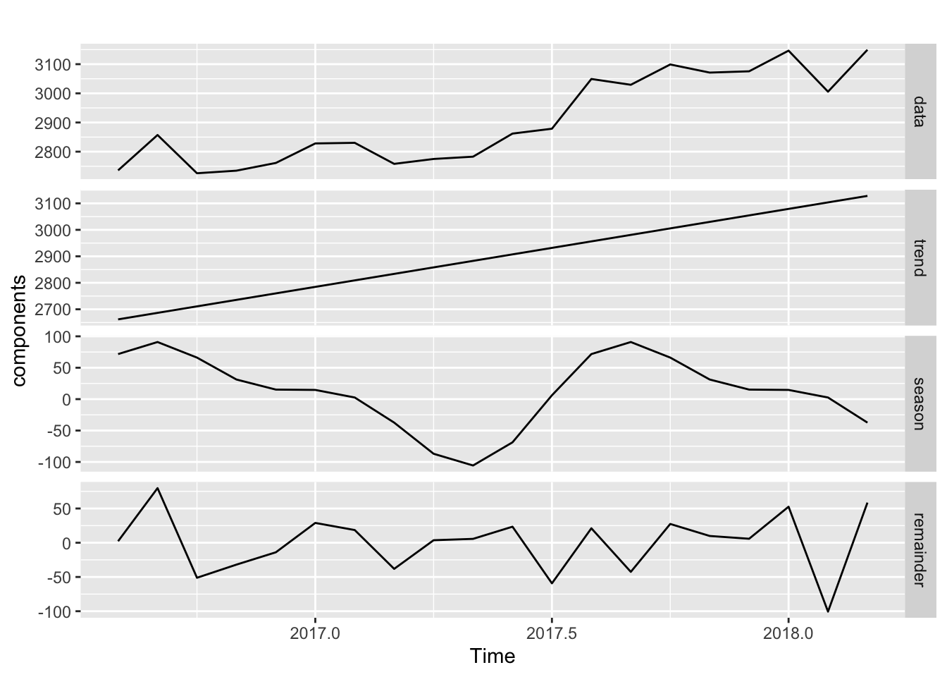

out <-forecast(decompose_df, newdata = df)

Warning in forecast.lm(decompose_df, newdata = df): newdata column names not
specified, defaulting to first variable required.

autoplot(out)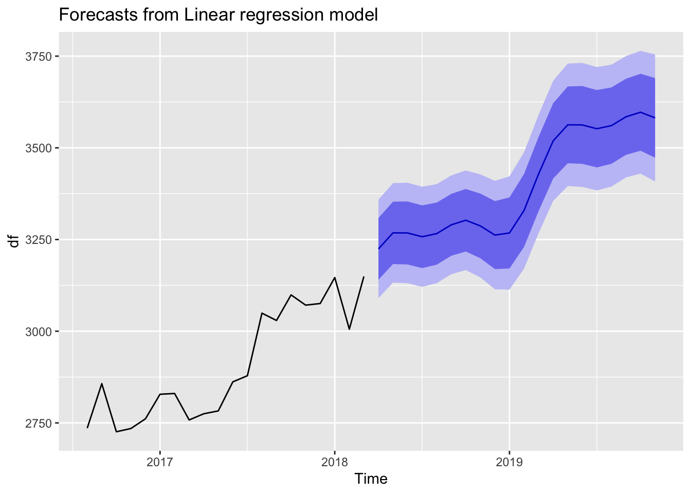

Footnotes

Read more about Fourier series and transforms on wikipedia. They are in my opinion a modern marvel of mathematics↩︎

Reuse

https://creativecommons.org/licenses/by/4.0/

Citation

BibTeX citation:

@online{dewitt2018,
  author = {Michael DeWitt and Michael DeWitt},
  title = {Analysis of {Short} {Time} {Series}},
  date = {2018-07-19},
  url = {https://michaeldewittjr.com/programming/2018-07-19-analysis-of-short-time-series},
  langid = {en}
}

For attribution, please cite this work as:

Michael DeWitt, and Michael DeWitt. 2018. “Analysis of Short Time Series.” July 19, 2018. https://michaeldewittjr.com/programming/2018-07-19-analysis-of-short-time-series.