library(deSolve)
library(tidyverse)2 The Basic Model of Virus Dynamics
Set Up the ODE
base_ode <- function(time, state, parameters){
    with(as.list(c(state, parameters)),{

        dx <- lambda - d*x - beta * x * v
        dy <- beta * x * v - a * y
        dv <- k * y - u * v

        return(list(c(dx,dy,dv)))
    })

}

t <- seq(0,30,.1)

params <- c(
    lambda =1e5,# Uninfected cell production rate
    d = .1, # Cell Death Rate
    a = .5, # Infected Cell Death Rate
    beta = 2e-7, # "Rate Constant"
    k = 100, # Virus productin from Infected cell
    u = 5 # Free Virus lifestapn
)
Guessing Initial values from a graph
x0 <- params["lambda"][1]/params["d"][1]
init <- c(x = unname(x0),
y = 1, v = 1)
out <- ode(init, t, base_ode, params)
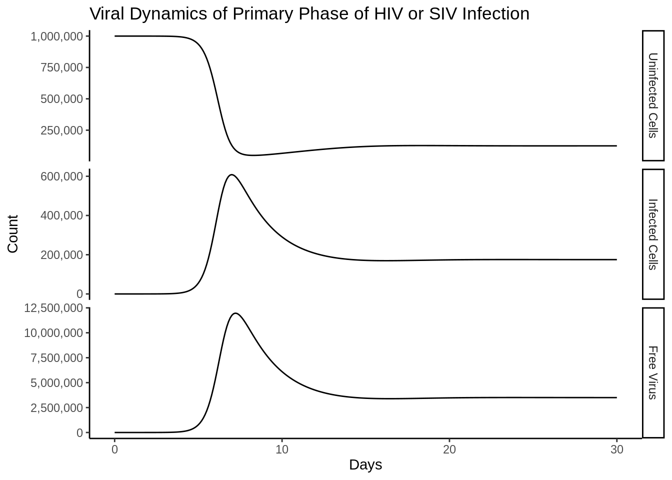
out_df <- as_tibble(as.data.frame(out))Funny side note is that the differences in the scales are almost immediately reproduced as in the book.
compartment_names <- c("Uninfected Cells",
"Infected Cells",
"Free Virus")

p <- out_df %>%
    setNames(c("time", compartment_names)) %>%
    gather(compartment, value, -time) %>%
    mutate(compartment = factor(compartment, compartment_names)) %>%
    ggplot(aes(time, y = value))+
    geom_line()+
    facet_grid(rows = vars(compartment),scales = "free_y")+
    theme_classic()+
    labs(
        title = "Viral Dynamics of Primary Phase of HIV or SIV Infection",
        x = "Days",
        y = "Count"
    )+
    scale_y_continuous(labels = scales::comma_format(accuracy = 1000))

p