Confirmatory Factor Analysis in Stan
The motivation for this post is to learn how to perform onfirmatory factor analysis(CFA) in Stan (and thus in a Bayesian way). These measures are typically noisey so Bayes, in my opinion, lends itself well to these kind of constructs. Additionaly, the gold standard for CFA in R is lavaan. This is nice because it provides a decent benchmark for the output of the Bayesian version. This post is largely inspired by the work done by Mike Lawrence on this topic here.
Data
The data that will be used will be that from the HolzingerSwineford1939 dataset that is part of the lavaan package.
library(lavaan)

HolzingerSwineford1939
Hypothesis Testing
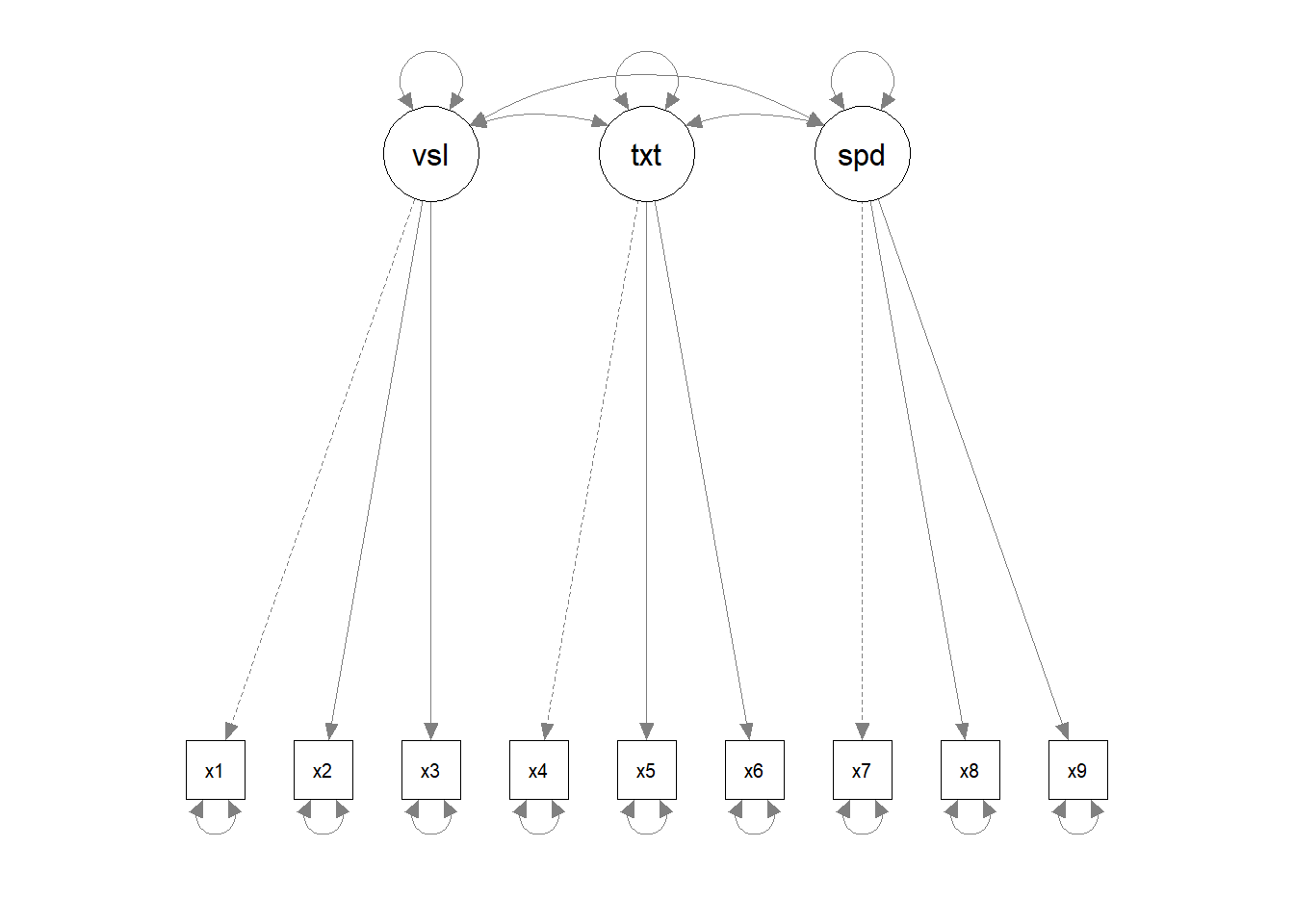
CFA differs from exploratory factor analysis (EFA) in the fact that one has a hypothesis for how the factors of a latent trait form. So the first step is to develop the hypothesised model:
Implmentation
Maximum Likelihood
Just to give the reference, first we will conduct the analysis in lavaan
cfa_model <- ' visual  =~ x1 + x2 + x3
              textual =~ x4 + x5 + x6
speed   =~ x7 + x8 + x9 '

cfa_fit <- cfa(cfa_model, HolzingerSwineford1939)
And we can examine the outputs:
summary(cfa_fit, fit.measures=TRUE)## lavaan 0.6-4 ended normally after 35 iterations
##
## Optimization method NLMINB
## Number of free parameters 21
##
## Number of observations 301
##
## Estimator ML
## Model Fit Test Statistic 85.306
## Degrees of freedom 24
## P-value (Chi-square) 0.000
##
## Model test baseline model:
##
## Minimum Function Test Statistic 918.852
## Degrees of freedom 36
## P-value 0.000
##
## User model versus baseline model:
##
## Comparative Fit Index (CFI) 0.931
## Tucker-Lewis Index (TLI) 0.896
##
## Loglikelihood and Information Criteria:
##
## Loglikelihood user model (H0) -3737.745
## Loglikelihood unrestricted model (H1) -3695.092
##
## Number of free parameters 21
## Akaike (AIC) 7517.490
## Bayesian (BIC) 7595.339
## Sample-size adjusted Bayesian (BIC) 7528.739
##
## Root Mean Square Error of Approximation:
##
## RMSEA 0.092
## 90 Percent Confidence Interval 0.071 0.114
## P-value RMSEA <= 0.05 0.001
##
## Standardized Root Mean Square Residual:
##
## SRMR 0.065
##
## Parameter Estimates:
##
## Information Expected
## Information saturated (h1) model Structured
## Standard Errors Standard
##
## Latent Variables:
## Estimate Std.Err z-value P(>|z|)
## visual =~
## x1 1.000
## x2 0.554 0.100 5.554 0.000
## x3 0.729 0.109 6.685 0.000
## textual =~
## x4 1.000
## x5 1.113 0.065 17.014 0.000
## x6 0.926 0.055 16.703 0.000
## speed =~
## x7 1.000
## x8 1.180 0.165 7.152 0.000
## x9 1.082 0.151 7.155 0.000
##
## Covariances:
## Estimate Std.Err z-value P(>|z|)
## visual ~~
## textual 0.408 0.074 5.552 0.000
## speed 0.262 0.056 4.660 0.000
## textual ~~
## speed 0.173 0.049 3.518 0.000
##
## Variances:
## Estimate Std.Err z-value P(>|z|)
## .x1 0.549 0.114 4.833 0.000
## .x2 1.134 0.102 11.146 0.000
## .x3 0.844 0.091 9.317 0.000
## .x4 0.371 0.048 7.779 0.000
## .x5 0.446 0.058 7.642 0.000
## .x6 0.356 0.043 8.277 0.000
## .x7 0.799 0.081 9.823 0.000
## .x8 0.488 0.074 6.573 0.000
## .x9 0.566 0.071 8.003 0.000
## visual 0.809 0.145 5.564 0.000
## textual 0.979 0.112 8.737 0.000
## speed 0.384 0.086 4.451 0.000Bayesian Version
Now first to write the Stan code:
library(rstan)
rstan_options(auto_write = TRUE)
writeLines(readLines("stan_cfa.stan"))
//confirmatory factor analysis code
data{
// n_subj: number of subjects
int n_subj ;
// n_y: number of outcomes
int n_y ;
// y: matrix of outcomes
matrix[n_subj,n_y] y ;
// n_fac: number of latent factors
int n_fac ;
// y_fac: list of which factor is associated with each outcome
int<lower=1,upper=n_fac> y_fac[n_y] ;
}
transformed data{
// scaled_y: z-scaled outcomes
matrix[n_subj,n_y] scaled_y ;
for(i in 1:n_y){
scaled_y[,i] = (y[,i]-mean(y[,i])) / sd(y[,i]) ;
}
}
parameters{
// normal01: a helper variable for more efficient non-centered multivariate
// sampling of subj_facs
matrix[n_fac, n_subj] normal01;
// fac_cor_helper: correlations (on cholesky factor scale) amongst latent
// factors
cholesky_factor_corr[n_fac] fac_cor_helper ;
// scaled_y_means: means for each outcome
vector[n_y] scaled_y_means ;
// scaled_y_noise: measurement noise for each outcome
vector<lower=0>[n_y] scaled_y_noise ;
// betas: how each factor loads on to each outcome.
// Must be postive for identifiability.
vector<lower=0>[n_y] betas ;
}
transformed parameters{
// subj_facs: matrix of values for each factor associated with each subject
matrix[n_subj,n_fac] subj_facs ;
// the following calculation implies that rows of subj_facs are sampled from
// a multivariate normal distribution with mean of 0 and sd of 1 in all
// dimensions and a correlation matrix of fac_cor.
subj_facs = transpose(fac_cor_helper * normal01) ;
}
model{
// normal01 must have normal(0,1) prior for "non-centered" parameterization
// on the multivariate distribution of latent factors
to_vector(normal01) ~ normal(0,1) ;
// flat prior on correlations
fac_cor_helper ~ lkj_corr_cholesky(1) ;
// normal prior on y means
scaled_y_means ~ normal(0,1) ;
// weibull prior on measurement noise
scaled_y_noise ~ weibull(2,1) ;
// normal(0,1) priors on betas
betas ~ normal(0,1) ;
// each outcome as normal, influenced by its associated latent factor
for(i in 1:n_y){
scaled_y[,i] ~ normal(
scaled_y_means[i] + subj_facs[,y_fac[i]] * betas[i]
, scaled_y_noise[i]
) ;
}
}
generated quantities{
//cors: correlations amongst within-subject predictors' effects
corr_matrix[n_fac] fac_cor ;
// y_means: outcome means on the original scale of Y
vector[n_y] y_means ;
// y_noise: outcome noise on the original scale of Y
vector[n_y] y_noise ;
fac_cor = multiply_lower_tri_self_transpose(fac_cor_helper) ;
for(i in 1:n_y){
y_means[i] = scaled_y_means[i]*sd(y[,i]) + mean(y[,i]) ;
y_noise[i] = scaled_y_noise[i]*sd(y[,i]) ;
}
}Then compile the model:
stan_cfa_model <- stan_model("stan_cfa.stan")Prep the Data
Of course with Stan we have to format our data. One note here is that we have to specify the parameters for our latent traits as well.
HolzingerSwineford1939 %>%
    dplyr::select(
        x1,x2,x3,x4,x5,x6,x7,x8,x9
    ) -> dat

stan_dat <- list(
    # n_y: number of outcomes
    n_y = ncol(dat)
    # n_subj: number of subjects
    , n_subj = nrow(dat)
    # y: matrix of outcomes
    , y = as.matrix(dat)
    # n_fac: number of latent factors
    , n_fac = 3
    # y_fac: list of which factor is associated with each outcome
    , y_fac = c(1,1,1,2,2,2,3,3,3)
)
Then run the model
stan_fit <- sampling(stan_cfa_model, stan_dat,
                     cores = 3, chains = 3, iter = 4000,
                     refresh = 0)
Let’s examine the convergence to make sure that enough iterations have been run.
traceplot(stan_fit)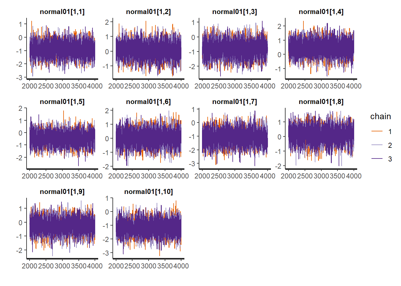
Not too bad. Now we can review our parameters
print(stan_fit, pars = c("betas", "fac_cor"))## Inference for Stan model: stan_cfa.
## 3 chains, each with iter=4000; warmup=2000; thin=1;
## post-warmup draws per chain=2000, total post-warmup draws=6000.
##
## mean se_mean sd 2.5% 25% 50% 75% 97.5% n_eff Rhat
## betas[1] 0.77 0 0.07 0.63 0.72 0.77 0.82 0.92 719 1
## betas[2] 0.42 0 0.07 0.29 0.38 0.42 0.47 0.56 2826 1
## betas[3] 0.58 0 0.07 0.45 0.53 0.58 0.63 0.72 1719 1
## betas[4] 0.85 0 0.05 0.76 0.82 0.85 0.89 0.95 2559 1
## betas[5] 0.86 0 0.05 0.76 0.83 0.86 0.89 0.96 2389 1
## betas[6] 0.84 0 0.05 0.75 0.81 0.84 0.87 0.94 2588 1
## betas[7] 0.56 0 0.07 0.42 0.52 0.56 0.61 0.70 1839 1
## betas[8] 0.72 0 0.08 0.56 0.67 0.72 0.77 0.87 905 1
## betas[9] 0.67 0 0.08 0.52 0.62 0.67 0.72 0.83 1215 1
## fac_cor[1,1] 1.00 NaN 0.00 1.00 1.00 1.00 1.00 1.00 NaN NaN
## fac_cor[1,2] 0.45 0 0.06 0.32 0.40 0.45 0.49 0.56 855 1
## fac_cor[1,3] 0.46 0 0.09 0.29 0.41 0.46 0.52 0.63 886 1
## fac_cor[2,1] 0.45 0 0.06 0.32 0.40 0.45 0.49 0.56 855 1
## fac_cor[2,2] 1.00 0 0.00 1.00 1.00 1.00 1.00 1.00 5768 1
## fac_cor[2,3] 0.28 0 0.07 0.13 0.23 0.28 0.32 0.41 2473 1
## fac_cor[3,1] 0.46 0 0.09 0.29 0.41 0.46 0.52 0.63 886 1
## fac_cor[3,2] 0.28 0 0.07 0.13 0.23 0.28 0.32 0.41 2473 1
## fac_cor[3,3] 1.00 0 0.00 1.00 1.00 1.00 1.00 1.00 5254 1
##
## Samples were drawn using NUTS(diag_e) at Tue Jul 16 08:24:46 2019.
## For each parameter, n_eff is a crude measure of effective sample size,
## and Rhat is the potential scale reduction factor on split chains (at
## convergence, Rhat=1).
Research and Methods Resources
me.dewitt.jr@gmail.com
Winston- Salem, NC
Copyright © 2018 Michael DeWitt. All rights reserved.