scd Micro Simulation
Introduction
The purpose of this simulation is to test the impact of statistical micro-discloure practices. Microdata are samples of the non-aggregated data (unit record) used for analysis. This is important in order to avoid the ecological inference problem1.
library(tidyverse)
library(sdcMicro)
## Registered S3 method overwritten by 'sets':
## method from
## print.element ggplot2## --------
## This is sdcMicro v5.4.0.
## For references, please have a look at citation('sdcMicro')
## Note: since version 5.0.0, the graphical user-interface is a shiny-app that can be started with sdcApp().
## Please submit suggestions and bugs at: https://github.com/sdcTools/sdcMicro/issues
## --------library(broom)Generate Known Data
As with any simulation or modeling process it is important to simulate some data with known parameters in order to better test the methods.
Population Parameters
Now to develop some synthetic data with some known population parameters.
set.seed(100)
gender_options <- c("M", "F")
gender_probs <- c(.4, .6)
race_options <- c("Asian", "Black/ African American","Hispanic", "White", "Other")
race_probs <- c(.07, .15, .15, .6,.03)
citizenship <- c("Y", "N", "RA")
citizenship_probs <- c(.9, .07, .03)
education <- c("HS", "Some College", "College", "Post-graduate")
education_probs <- c(.35, .35, .25, .05)
Generate the Data
dat_1 <- data.frame(
  gender = sample( 500, x = gender_options, replace = T, prob = gender_probs),
  race = sample( 500, x = race_options, replace = T, prob = race_probs),
  citizenship = sample(500, x = citizenship, replace = T, prob = citizenship_probs),
  education = sample( 500, x = education, replace = T, prob = education_probs),
  income = rbeta(500, shape1 = 1, 5)*100000,
  debt = rnorm(500, mean = 20000, 5000)
) %>%
  mutate(id = row_number()) %>%
  mutate_if(is.character, as.factor)

dat_2 <- dat_1 %>%
  mutate(citizenship = fct_lump(citizenship, 1))
Examine the Real Data Cross Tabs
dat_1 %>%
  group_by(gender, race) %>%
  summarise(avg_income = mean(income)) %>%
  spread(gender, avg_income)
Statistical Disclosure Methods
Now we can explore the sdcMicro package with some additional details.
Assess the Risk
I am going to declare the race, gender, citizenship, education, income and debt are all sensitive variables. I can then perform the freqCalc to see if there are unique and identifying combinations of these parameters in the data.
key_vars <- c("race", "gender", "citizenship", "education")
conti_vars <- c("income", "debt")
(initial_fc <- freqCalc(dat_1, keyVars = key_vars))
##
## --------------------------
## 28 obs. violate 2-anonymity
## 42 obs. violate 3-anonymity
## --------------------------Now Make the sdcMicro Object
For best use of the package, it is important to create an Sdc object with the specified important or sensitive variables
sdc_micro <- createSdcObj(dat_2,
                          keyVars = key_vars,
                          numVars =conti_vars,
                          pramVars = key_vars)
Now we can examine the outputted object:
sdc_micro## The input dataset consists of 500 rows and 7 variables.
## --> Categorical key variables: race, gender, citizenship, education
## --> Numerical key variables: income, debt
## ----------------------------------------------------------------------
##
## Information on categorical key variables:
##
## Reported is the number, mean size and size of the smallest category for recoded variables.
## In parenthesis, the same statistics are shown for the unmodified data.
## Note: NA (missings) are counted as seperate categories!
##
## Key Variable Number of categories Mean size
## race 5 (5) 100.000 (100.000)
## gender 2 (2) 250.000 (250.000)
## citizenship 2 (2) 250.000 (250.000)
## education 4 (4) 125.000 (125.000)
## Size of smallest
## 18 (18)
## 203 (203)
## 56 (56)
## 29 (29)
## ----------------------------------------------------------------------
##
## Infos on 2/3-Anonymity:
##
## Number of observations violating
## - 2-anonymity: 18 (3.600%)
## - 3-anonymity: 36 (7.200%)
## - 5-anonymity: 67 (13.400%)
##
## ----------------------------------------------------------------------
##
## Numerical key variables: income, debt
##
## Disclosure risk is currently between [0.00%; 100.00%]
##
## Current Information Loss:
## - IL1: 0.00
## - Difference of Eigenvalues: 0.000%
## ----------------------------------------------------------------------Handle Categorical
Now we can apply some methods to mask some of the categorical variables. Additionally, from the output one can gather how much the data has changed.
(clean_1 <- sdcMicro::pram(sdc_micro))## Warning in pramX(obj = obj, variables = variables, strata_variables = strata_variables, : If pram is applied on key variables, the k-anonymity and risk assessment are not useful anymore.## The input dataset consists of 500 rows and 7 variables.
## --> Categorical key variables: race, gender, citizenship, education
## --> Numerical key variables: income, debt
## ----------------------------------------------------------------------
##
## Information on categorical key variables:
##
## Reported is the number, mean size and size of the smallest category for recoded variables.
## In parenthesis, the same statistics are shown for the unmodified data.
## Note: NA (missings) are counted as seperate categories!
##
## Key Variable Number of categories Mean size
## race 5 (5) 100.000 (100.000)
## gender 2 (2) 250.000 (250.000)
## citizenship 2 (2) 250.000 (250.000)
## education 4 (4) 125.000 (125.000)
## Size of smallest
## 18 (18)
## 198 (203)
## 56 (56)
## 27 (29)
## ----------------------------------------------------------------------
##
## Infos on 2/3-Anonymity:
##
## Number of observations violating
## - 2-anonymity: 13 (2.600%) | in original data: 18 (3.600%)
## - 3-anonymity: 33 (6.600%) | in original data: 36 (7.200%)
## - 5-anonymity: 68 (13.600%) | in original data: 67 (13.400%)
##
## ----------------------------------------------------------------------
##
## Numerical key variables: income, debt
##
## Disclosure risk (~100.00% in original data):
## modified data: [0.00%; 100.00%]
##
## Current Information Loss in modified data (0.00% in original data):
## IL1: 0.00
## Difference of Eigenvalues: 0.000%
## ----------------------------------------------------------------------
##
## Post-Randomization (PRAM):
## Variable: race
## --> final Transition-Matrix:
## Asian Black/ African American Hispanic
## Asian 0.85218646 0.003204457 0.02664387
## Black/ African American 0.00147028 0.923191882 0.01349424
## Hispanic 0.01282853 0.014160620 0.87351742
## Other 0.01819908 0.019061417 0.05640076
## White 0.01542621 0.017738630 0.02542872
## Other White
## Asian 0.008399576 0.10956564
## Black/ African American 0.004036535 0.05780706
## Hispanic 0.012533501 0.08695993
## Other 0.714192700 0.19214605
## White 0.012486025 0.92892042
## Variable: gender
## --> final Transition-Matrix:
## F M
## F 0.9227536 0.07724644
## M 0.1130157 0.88698428
## Variable: citizenship
## --> final Transition-Matrix:
## Y Other
## Y 0.9647225 0.03527748
## Other 0.2797000 0.72029998
## Variable: education
## --> final Transition-Matrix:
## College HS Post-graduate Some College
## College 0.96023128 0.02651010 0.006111854 0.007146767
## HS 0.01786242 0.95667024 0.011635183 0.013832152
## Post-graduate 0.02655495 0.07502687 0.890021347 0.008396827
## Some College 0.00569932 0.01637097 0.001541190 0.976388525
##
## Changed observations:
## variable nrChanges percChanges
## 1 race 52 10.4
## 2 gender 33 6.6
## 3 citizenship 32 6.4
## 4 education 16 3.2
## ----------------------------------------------------------------------Handle Numeric
(clean_2 <- microaggregation(clean_1, method = "rmd", aggr = 3))## The input dataset consists of 500 rows and 7 variables.
## --> Categorical key variables: race, gender, citizenship, education
## --> Numerical key variables: income, debt
## ----------------------------------------------------------------------
##
## Information on categorical key variables:
##
## Reported is the number, mean size and size of the smallest category for recoded variables.
## In parenthesis, the same statistics are shown for the unmodified data.
## Note: NA (missings) are counted as seperate categories!
##
## Key Variable Number of categories Mean size
## race 5 (5) 100.000 (100.000)
## gender 2 (2) 250.000 (250.000)
## citizenship 2 (2) 250.000 (250.000)
## education 4 (4) 125.000 (125.000)
## Size of smallest
## 18 (18)
## 198 (203)
## 56 (56)
## 27 (29)
## ----------------------------------------------------------------------
##
## Infos on 2/3-Anonymity:
##
## Number of observations violating
## - 2-anonymity: 13 (2.600%) | in original data: 18 (3.600%)
## - 3-anonymity: 33 (6.600%) | in original data: 36 (7.200%)
## - 5-anonymity: 68 (13.600%) | in original data: 67 (13.400%)
##
## ----------------------------------------------------------------------
##
## Numerical key variables: income, debt
##
## Disclosure risk (~100.00% in original data):
## modified data: [0.00%; 77.80%]
##
## Current Information Loss in modified data (0.00% in original data):
## IL1: 11898.92
## Difference of Eigenvalues: 0.100%
## ----------------------------------------------------------------------
##
## Post-Randomization (PRAM):
## Variable: race
## --> final Transition-Matrix:
## Asian Black/ African American Hispanic
## Asian 0.85218646 0.003204457 0.02664387
## Black/ African American 0.00147028 0.923191882 0.01349424
## Hispanic 0.01282853 0.014160620 0.87351742
## Other 0.01819908 0.019061417 0.05640076
## White 0.01542621 0.017738630 0.02542872
## Other White
## Asian 0.008399576 0.10956564
## Black/ African American 0.004036535 0.05780706
## Hispanic 0.012533501 0.08695993
## Other 0.714192700 0.19214605
## White 0.012486025 0.92892042
## Variable: gender
## --> final Transition-Matrix:
## F M
## F 0.9227536 0.07724644
## M 0.1130157 0.88698428
## Variable: citizenship
## --> final Transition-Matrix:
## Y Other
## Y 0.9647225 0.03527748
## Other 0.2797000 0.72029998
## Variable: education
## --> final Transition-Matrix:
## College HS Post-graduate Some College
## College 0.96023128 0.02651010 0.006111854 0.007146767
## HS 0.01786242 0.95667024 0.011635183 0.013832152
## Post-graduate 0.02655495 0.07502687 0.890021347 0.008396827
## Some College 0.00569932 0.01637097 0.001541190 0.976388525
##
## Changed observations:
## variable nrChanges percChanges
## 1 race 52 10.4
## 2 gender 33 6.6
## 3 citizenship 32 6.4
## 4 education 16 3.2
## ----------------------------------------------------------------------For the final step we can pull the new data out of the sdc object.
anon_data <- extractManipData(clean_2)Compare New Data with True
Now we can perform some regressions using the true data and the perturbed data to examine the different results.
options(digits =2)
fit_1 <- lm(income~ race + education + citizenship, data = dat_2)
fit_2 <- lm(income~ race + education + citizenship, data = anon_data)

tidy(fit_1) %>%
  dplyr::select(term, estimate) %>%
  rename(original_data = estimate) %>%
  cbind(tidy(fit_2) %>% dplyr::select(estimate)) %>%
  rename(anon_data = estimate) %>%
  mutate(delta = original_data - anon_data) %>%
knitr::kable(digits = 2)| term | original_data | anon_data | delta |
|---|---|---|---|
| (Intercept) | 13418 | 15949 | -2531 |
| raceBlack/ African American | 1982 | 309 | 1673 |
| raceHispanic | 2063 | 814 | 1250 |
| raceOther | 4156 | -583 | 4740 |
| raceWhite | 2096 | -1002 | 3097 |
| educationHS | 1778 | 1448 | 330 |
| educationPost-graduate | 1320 | 2467 | -1147 |
| educationSome College | 1786 | 1570 | 216 |
| citizenshipOther | 3324 | 3270 | 54 |
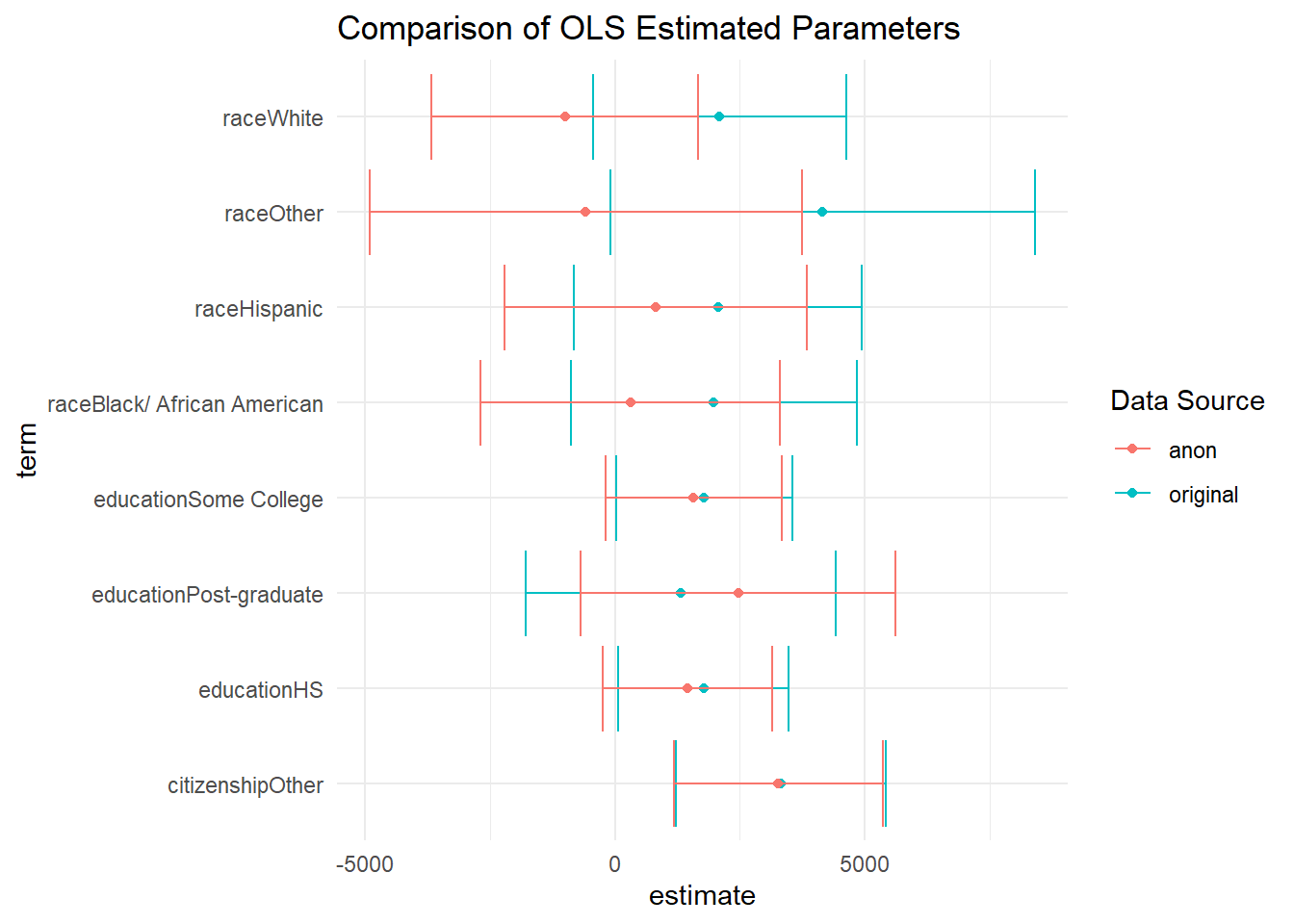
In general the signs of the regression are all consistent. The magnitude of the effects have changed slightly. We can plot the outputs to get a better idea of these differences.
fit_1_broom <- tidy(fit_1) %>%
  mutate(id = "original")
fit_2_broom <- tidy(fit_2) %>%
  mutate(id = "anon")

combined_dat <- bind_rows(fit_1_broom, fit_2_broom)

combined_dat %>%
  filter(!grepl("(Intercept)", term)) %>%
  ggplot(aes(term, estimate, group = id, color = id))+
  geom_point()+
  geom_errorbar(aes(ymin = estimate - std.error,
                    ymax = estimate + std.error))+
  theme_minimal()+
  coord_flip()+
  labs(
    title = "Comparison of OLS Estimated Parameters",
    color = "Data Source"
  )
sdcMicro::calcRisks(clean_2)## The input dataset consists of 500 rows and 7 variables.
## --> Categorical key variables: race, gender, citizenship, education
## --> Numerical key variables: income, debt
## ----------------------------------------------------------------------
##
## Information on categorical key variables:
##
## Reported is the number, mean size and size of the smallest category for recoded variables.
## In parenthesis, the same statistics are shown for the unmodified data.
## Note: NA (missings) are counted as seperate categories!
##
## Key Variable Number of categories Mean size
## race 5 (5) 100.000 (100.000)
## gender 2 (2) 250.000 (250.000)
## citizenship 2 (2) 250.000 (250.000)
## education 4 (4) 125.000 (125.000)
## Size of smallest
## 18 (18)
## 198 (203)
## 56 (56)
## 27 (29)
## ----------------------------------------------------------------------
##
## Infos on 2/3-Anonymity:
##
## Number of observations violating
## - 2-anonymity: 13 (2.600%) | in original data: 18 (3.600%)
## - 3-anonymity: 33 (6.600%) | in original data: 36 (7.200%)
## - 5-anonymity: 68 (13.600%) | in original data: 67 (13.400%)
##
## ----------------------------------------------------------------------
##
## Numerical key variables: income, debt
##
## Disclosure risk (~100.00% in original data):
## modified data: [0.00%; 77.80%]
##
## Current Information Loss in modified data (0.00% in original data):
## IL1: 11898.92
## Difference of Eigenvalues: 0.100%
## ----------------------------------------------------------------------
##
## Post-Randomization (PRAM):
## Variable: race
## --> final Transition-Matrix:
## Asian Black/ African American Hispanic Other
## Asian 0.8522 0.0032 0.027 0.0084
## Black/ African American 0.0015 0.9232 0.013 0.0040
## Hispanic 0.0128 0.0142 0.874 0.0125
## Other 0.0182 0.0191 0.056 0.7142
## White 0.0154 0.0177 0.025 0.0125
## White
## Asian 0.110
## Black/ African American 0.058
## Hispanic 0.087
## Other 0.192
## White 0.929
## Variable: gender
## --> final Transition-Matrix:
## F M
## F 0.92 0.077
## M 0.11 0.887
## Variable: citizenship
## --> final Transition-Matrix:
## Y Other
## Y 0.96 0.035
## Other 0.28 0.720
## Variable: education
## --> final Transition-Matrix:
## College HS Post-graduate Some College
## College 0.9602 0.027 0.0061 0.0071
## HS 0.0179 0.957 0.0116 0.0138
## Post-graduate 0.0266 0.075 0.8900 0.0084
## Some College 0.0057 0.016 0.0015 0.9764
##
## Changed observations:
## variable nrChanges percChanges
## 1 race 52 10.4
## 2 gender 33 6.6
## 3 citizenship 32 6.4
## 4 education 16 3.2
## ----------------------------------------------------------------------Match Anon Data Back to Original Data
Now let’s see if I can match this data back. I’ll use the fastLink package to see if I can link some of the masked data back to the original data set. I’ll also use the original key values which represents the worst case where an intruder would have access to all of these key variables.
library(fastLink)

matching_test <- fastLink(dfA = anon_data,
                          dfB = dat_1,
                          varnames = key_vars, n.cores = 3, verbose = FALSE)
##
## ====================
## fastLink(): Fast Probabilistic Record Linkage
## ====================
##
## Calculating matches for each variable.
## Getting counts for parameter estimation.
## Parallelizing calculation using OpenMP. 1 threads out of 4 are used.
## Running the EM algorithm.
## Getting the indices of estimated matches.
## Parallelizing calculation using OpenMP. 1 threads out of 4 are used.
## Deduping the estimated matches.
## Getting the match patterns for each estimated match.Now let’s returned the matched data frame. I will use a 95% confidence level for returning matches.
matched_dfs <- getMatches(
  dfA = anon_data, dfB = dat_1,
  fl.out = matching_test, threshold.match = 0.95
)
We can then see our accuracy at matching
options(digits = 2)
df <- matching_test$matches

mean(df[["inds.a"]] == df[["inds.b"]])
## [1] 0.065Thus only 6.5% were actually identified. Of those we can see how many were uniquely matched
df %>%
  count(inds.b) %>%
  left_join(filter(df, inds.a==inds.b)) %>%
  filter(!is.na(inds.a), n == 1)
## Joining, by = "inds.b"Therefore 17 out of 500 or 3.4% were uniquely identified. Now more modifications could be done to improve the masking of the data.
Research and Methods Resources
me.dewitt.jr@gmail.com
Winston- Salem, NC
Copyright © 2018 Michael DeWitt. All rights reserved.