Data Cleaning
Wide to Long, Long to Wide
As discussed in the slides, we will use functions from tidyr (automatically loaded with the tidyverse) to manipulate our data.
gather for wide to narrow
Let’s read in our data set.
First we need to call in our libraries:
library(tidyverse)Now we can read in our data using readr’s read_csv function
gap_wide <- read_csv("data/gapminder_wide.csv")## Parsed with column specification:
## cols(
## .default = col_integer()
## )## See spec(...) for full column specifications.Go ahead and look at the data in the environment pane
Tidy it up
Now we need to use the gather function:
gap_narrow <- gap_wide %>%
  gather(key = "country", value = "population", -year)
Now we can inspect our work:
head(gap_narrow)As a teaser, this can be used to make some very slick graphics
gap_narrow %>%
  filter(country %in% c("India", "China", "Germany", "France")) %>%
  ggplot(aes(year, population))+
  geom_smooth()+
  facet_wrap(~country)
## `geom_smooth()` using method = 'loess' and formula 'y ~ x'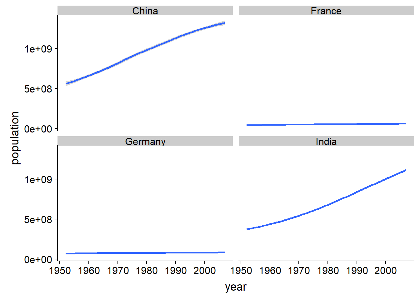
Now To Spread with spread
Sometimes data come in a long format where it needs to be a little wider to fit our tidy paradigm.
Let’s experiment with spreading data. Let’s read in the health_long.xlsx file from our data folder.
This requires the readxl package.
library(readxl)Now let’s read it into memory.
health_long <- read_excel("data/health_long.xlsx")We can look at the format of the data
head(health_long)It appears that each subject appears in multiple rows with repeating attributes in the “measurement” column.
Thus we want to spread measurement (which will make new column names) and then have the values in these new columns be those values in the value column.
health_long %>%
  spread(key = measurement, value = value)
Exercise 1 - Your Turn!
Read in the heights.dta file. This file contains data on some physical attributes and earnings of subjects in a study.
Hint: you will need to use the haven package. Put the data into a tidy format. You will note that it is currently in a long format.
read in the data
library(haven)
heights_raw <- read_dta("data/heights.dta")
tidy it
Long -> Wide
heights_raw %>%
  spread(key = description, value = value, fill = NA)
Exercise 2
Read in the gapminder.sav data set and collapse all the metrics for life expectancy, population and GDP per Population into two columns one for parameter_name and the other for value.
gapminder<-read_sav("data/gapminder.sav")Hint: you will need to use the -group_1, -group_2, etc syntax to not collapse the grouping variables that you wish to keep.
gapminder %>%
  gather(key = parameter_name, value = value, -country, -continent, -year)
## Warning: attributes are not identical across measure variables;
## they will be droppedExcerise 3
Using select to subset
From the gapminder data set that you already read into memory, select the “year” and “pop” columns
gapminder %>%
  select(year, pop)
Excerise 4
Use the unite function to combine “year” and “country” into one column called country_year with values separated by a “-”. Save this into an object called “unite_demo.”
# In this case I will specify the two columns I want to joinh
# Equivalently I could have used the -lifeExp, -Continent, -pop, -gpdPercap and gotten the same results
unite_demo <- gapminder %>%
  unite(country_year, sep = "-", c(year, country))

unite_demo
Exercise 5
Now convert this new data set back into the “year” and “country” columns using separate.
unite_demo %>%
  separate(col = country_year, into = c("country", "year"), sep = "-")
Exercise 6
Now let’s return to the gap_narrow dataset and filter the “year” field for values for “1977” only using the filter function and the == operator
gap_narrow %>%
  filter(year == 1977)
Bonus
Using the gap_narrow dataset let’s print the row with the maximum population.
Exercise 7
Let’s combine a few operations together using the pipe %>%.
Take the “health_long” data set
spreadto a tidy formatrenamethe “subject” column to “subject_id”use
mutateto create a value for total cholesterol (e.g. total_cholesterol = lhl + hdl)
health_long %>%
  spread(key = measurement, value = value, fill = NA) %>%
  rename(subject_id = subject) %>%
  mutate(total_cholesterol = ldl + hdl)
Of course if I want to write this data out I can do so:
my_new_health_data <- health_long %>%
  spread(key = measurement, value = value, fill = NA) %>%
  rename(subject_id = subject) %>%
  mutate(total_cholesterol = ldl + hdl)

write_csv(my_new_health_data, "outputs/my_new_health_data.csv")
Bonus
I discussed group_by for group-wise operations. Taking our gapminder data we could summarise the world population by year.
gapminder %>%
  group_by(year) %>%
  summarise(total_pop = max(pop))
Or by year and continent:
gapminder %>%
  group_by(year, continent) %>%
  summarise(total_pop = max(pop))
This then lets us do some neat graphing
gapminder %>%
  group_by(year, continent) %>%
  summarise(total_pop = max(pop)) %>%
  ggplot(aes(year, total_pop,
             group = continent, color = as_factor(continent)))+
  geom_line()+
  scale_y_log10()+
  labs(
    title = "Population Trends Over Time",
    subtitle = "From The Hans Rosling's Gapminder Dataset",
    y = "Population (log10)",
    x = NULL,
    color = "Continent"
  )+
  theme_minimal()
## Don't know how to automatically pick scale for object of type labelled. Defaulting to continuous.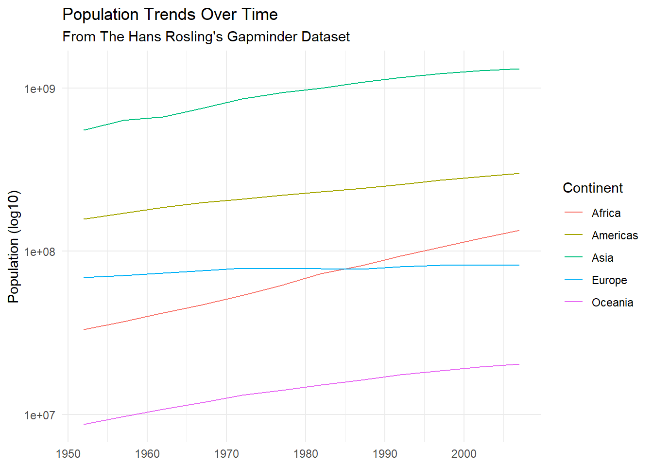
Introduction to R
dewittme.wfu.edu
Office of Institutional Research
309 Reynolda Hall
Winston- Salem, NC, 27106
Copyright © 2018 Michael DeWitt. All rights reserved.